View on GitHub Download .py

LC10a and LC9 output clusters

Introduction

Question

Do the LC10a and LC9 cells split into groups by their strong output connectivity, and do the groups view different regions of the eye?

Background

The dendrites of one LC type sit in the lobula, where each cell covers part of the visual field and the cells together cover all of it:

individual dendritic arbors spread across only part of the array of lobula columns but which, with a few exceptions, cover the entire visual field as a population

— Wu et al. 2016, p. 2 · PDF p. 2 · 10.7554/eLife.21022

Two cells of the same type can therefore view different regions. If their outputs follow that position, cells that view the same region drive the same partners and cells that view different regions do not. The axons of the LC types keep some of the position:

axonal projections of LC neurons to the AOTu retain retinotopy for azimuthal positions

— Wu et al. 2016, p. 5 · PDF p. 5 · 10.7554/eLife.21022

and for LC9 in particular:

terminals of single LC9 cells expanded through only part of the glomerulus and their position correlated with the approximate position of the corresponding dendrites in the lobula

— Wu et al. 2016, p. 10 · PDF p. 10 · 10.7554/eLife.21022

Dr. Chiappe suggested that each type has sub-populations that view different regions of the visual field (frontal, lateral, posterior) and drive different sets of postsynaptic cells, and that later comparisons of convergence should pair the sub-populations that view the same region instead of whole types. This notebook asks whether the connectivity shows such groups. It uses the right hemisphere only, the better-proofread side, and the strong partners of lc_output_strength, the proofread partners with a strength of at least STRONG_SYN = 10, with the LC cells among them removed.

Expectations

1. Without distinct groups, a type is a continuum: any clustering cuts it at arbitrary places, so the silhouette of a clustering is low and two clustering methods do not agree on the labels. With groups, there is a number of clusters \(k > 1\) at which two methods agree, which this notebook takes as an adjusted Rand index of at least AGREE_ARI = 0.5.
2. Without a link to position, a cluster spreads over the region bins about evenly, each holding about 33% of its cells. With a link, some clusters sit almost entirely in one bin of an address coordinate, at least PURE_SHARE = 90% of their cells.

Load data

The analysis reads census, which gives each cell's type, sides, which says which hemisphere a cell is in, proofread_ids, which lists the proofread neurons, and columns, the visual-column address \((x, y)\) of the columnar cells.

census = load_census()
census

shape: (138_327, 2)

root_id	primary_type
i64	str
720575940599457990	"T4b"
720575940599763910	"T5b"
720575940600623020	"Dm3q"
720575940602564320	"KCg-m"
720575940602720940	"JO-CA"
…	…
720575940661275009	"KCab-p"
720575940661281409	"L4"
720575940661285249	"LPC2"
720575940661304449	"Lawf1"
720575940661333889	"CB2303"

sides = load_visual_types().select("root_id", "side")
sides

shape: (95_079, 2)

root_id	side
i64	str
720575940596125868	"right"
720575940597856265	"right"
720575940597944841	"right"
720575940598267657	"right"
720575940599333574	"right"
…	…
720575940661323905	"left"
720575940661325697	"left"
720575940661327745	"right"
720575940661336193	"left"
720575940661339777	"right"

proofread_ids = load_proofread_ids()
proofread_ids

shape: (139_255, 1)

root_id
i64
720575940599457990
720575940599763910
720575940600623020
720575940602309600
720575940602564320
…
720575940661275009
720575940661281409
720575940661285249
720575940661304449
720575940661333889

columns = load_columns()
columns

shape: (45_528, 8)

root_id	hemisphere	type	column_id	x	y	p	q
i64	str	str	i64	i64	i64	i64	i64
720575940596125868	"right"	"T5c"	97	-5	2	6	-4
720575940599333574	"right"	"Tm1"	355	-7	-6	4	-10
720575940599457990	"right"	"T4b"	247	-4	-15	-4	-11
720575940599459782	"right"	"T5b"	513	-4	-13	-3	-10
720575940599704006	"right"	"T5a"	331	1	-15	-9	-6
…	…	…	…	…	…	…	…
720575940661281409	"left"	"L4"	385	-3	-18	-6	-12
720575940661284993	"right"	"R8"	694	4	3	-3	6
720575940661297281	"left"	"Tm21"	514	-4	-10	-1	-9
720575940661319553	"left"	"L3"	634	-3	-15	-5	-10
720575940661323905	"left"	"L4"	647	-4	-7	0	-7

The types are restricted to the right hemisphere.

cells = cells_of_types(census, sides, TYPES)
pl.DataFrame(
    {
        "type": list(TYPES),
        "right-hemisphere cells": [len(cells[_t]) for _t in TYPES],
    }
)

shape: (2, 2)

type	right-hemisphere cells
str	i64
"LC10a"	121
"LC9"	92

connections has one row per connection that starts at one of those cells, with its weight and the type of its presynaptic cell (pre_type). inputs has the connections that end at those cells and start at a columnar cell, which give each cell its address below.

_scored = [_id for _ids in cells.values() for _id in _ids]
connections = with_pre_type(load_connections_of(_scored), cells)
connections

shape: (121_285, 4)

pre_pt_root_id	post_pt_root_id	weight	pre_type
i64	i64	i64	str
720575940604681830	720575940379851795	1	"LC9"
720575940604681830	720575940379877395	1	"LC9"
720575940604681830	720575940379881235	1	"LC9"
720575940604681830	720575940379890707	1	"LC9"
720575940604681830	720575940379907789	1	"LC9"
…	…	…	…
720575940658842753	720575940643127319	1	"LC10a"
720575940658842753	720575940645579556	27	"LC10a"
720575940658842753	720575940646350702	3	"LC10a"
720575940658842753	720575940647062580	1	"LC10a"
720575940658842753	720575940647291427	1	"LC10a"

_scored = [_id for _ids in cells.values() for _id in _ids]
_columnar = set(columns["root_id"].to_list())
inputs = load_connections_of(_scored, end="post").filter(
    pl.col("pre_pt_root_id").is_in(list(_columnar))
)
inputs

shape: (3_381, 3)

pre_pt_root_id	post_pt_root_id	weight
i64	i64	i64
720575940602572768	720575940607839189	1
720575940602572768	720575940624856112	2
720575940602572768	720575940626008153	1
720575940602572768	720575940632871905	2
720575940602572768	720575940639702581	1
…	…	…
720575940659975297	720575940625772943	1
720575940659975297	720575940637379517	1
720575940659978625	720575940633523100	1
720575940660628609	720575940628679887	2
720575940660865409	720575940629817849	3

partners is the table of lc_output_strength (strengths_to_partners_with_cell_fraction, then label_partners), and strong_sets lists the ids of the strong partners of each type, as its strong_set takes them: the proofread partners with a strength of at least STRONG_SYN, without the LC cells among them.

partners = label_partners(
    strengths_to_partners_with_cell_fraction(connections, cells),
    census,
    proofread_ids,
)
partners

shape: (77_954, 9)

type	partner	s	synapses	cells	cell_fraction	partner_type	proofread	lateral
str	i64	i64	i64	u32	f64	str	bool	bool
"LC10a"	720575940379710175	1	1	1	0.008264	"unproofread fragment"	false	false
"LC10a"	720575940379714527	1	1	1	0.008264	"unproofread fragment"	false	false
"LC10a"	720575940379724716	1	1	1	0.008264	"unproofread fragment"	false	false
"LC10a"	720575940379730143	1	1	1	0.008264	"unproofread fragment"	false	false
"LC10a"	720575940379737004	1	1	1	0.008264	"unproofread fragment"	false	false
…	…	…	…	…	…	…	…	…
"LC9"	720575940660758401	1	1	1	0.01087	"Li08"	true	false
"LC9"	720575940661134465	2	4	3	0.032609	"Li06"	true	false
"LC9"	720575940661244033	2	2	1	0.01087	"TmY15"	true	false
"LC9"	720575940661318017	2	5	3	0.032609	"LLPC3"	true	false
"LC9"	720575940661327745	1	1	1	0.01087	"LTe09"	true	false

strong_sets = {
    _t: strong_set(partners)
    .filter(pl.col("type") == _t)["partner"]
    .sort()
    .to_list()
    for _t in TYPES
}
pl.DataFrame(
    {
        "type": list(TYPES),
        "strong partners": [len(strong_sets[_t]) for _t in TYPES],
    }
)

shape: (2, 2)

type	strong partners
str	i64
"LC10a"	85
"LC9"	89

Output profiles

The output profile of a cell is its weight onto each strong partner of its type, divided by its total over those partners, so that a profile is a distribution over partners and the total output of a cell does not dominate the distance between two cells. A cell with no strong partner has a profile of zeros. output_profiles returns a Profiles with the cells, the partners, and the matrix, one row per cell. On four connections of two cells onto three partners:

class Profiles(NamedTuple):
    """The output profiles of some cells.

    cells and partners are the root ids of the rows and the columns of
    matrix, and each row of matrix is a distribution over the partners,
    or zeros for a cell with no connection to them.
    """

    cells: list[int]
    partners: list[int]
    matrix: np.ndarray

def output_profiles(
    connections: pl.DataFrame, cells: list[int], partners: list[int]
) -> Profiles:
    """The output profile of each cell of cells over partners.

    connections is DataFrame[pre_pt_root_id, post_pt_root_id, weight];
    a connection that does not start at a cell or end at a partner is
    ignored.
    """
    cell_row = {cell: row for row, cell in enumerate(cells)}
    partner_column = {partner: col for col, partner in enumerate(partners)}
    kept = connections.filter(
        pl.col("pre_pt_root_id").is_in(cells)
        & pl.col("post_pt_root_id").is_in(partners)
    )
    matrix = np.zeros((len(cells), len(partners)))
    np.add.at(
        matrix,
        (
            [cell_row[c] for c in kept["pre_pt_root_id"]],
            [partner_column[p] for p in kept["post_pt_root_id"]],
        ),
        kept["weight"].to_numpy(),
    )
    totals = matrix.sum(axis=1, keepdims=True)
    return Profiles(
        cells=list(cells),
        partners=list(partners),
        matrix=np.divide(
            matrix, totals, out=np.zeros_like(matrix), where=totals > 0
        ),
    )

output_profiles(
    pl.DataFrame(
        {
            "pre_pt_root_id": [1, 1, 2, 2],
            "post_pt_root_id": [10, 11, 11, 12],
            "weight": [3, 1, 2, 2],
        }
    ),
    cells=[1, 2],
    partners=[10, 11, 12],
)

Profiles(cells=[1, 2], partners=[10, 11, 12], matrix=array([[0.75, 0.25, 0.  ],
       [0.  , 0.5 , 0.5 ]]))

The profiles of the real cells, with the cells that have no strong output:

profiles = {
    _t: output_profiles(connections, cells[_t], strong_sets[_t])
    for _t in TYPES
}
pl.DataFrame(
    {
        "type": list(TYPES),
        "cells": [len(profiles[_t].cells) for _t in TYPES],
        "strong partners": [len(profiles[_t].partners) for _t in TYPES],
        "cells with no strong output": [
            int((profiles[_t].matrix.sum(axis=1) == 0).sum())
            for _t in TYPES
        ],
    }
)

shape: (2, 4)

type	cells	strong partners	cells with no strong output
str	i64	i64	i64
"LC10a"	121	85	0
"LC9"	92	89	0

Two clusterings

Several methods suit a sparse profile matrix. Two with different assumptions are run, and their agreement is the evidence. k-means minimizes the squared Euclidean distance of the profiles to the center of their cluster. Agglomerative clustering merges the closest two clusters until \(k\) remain, with cosine distance between profiles and average linkage between clusters. Each takes the number of clusters \(k\). On four profiles that split in two:

def kmeans_labels(
    matrix: np.ndarray, k: int, *, seed: int = RANDOM_STATE
) -> np.ndarray:
    """The k-means cluster of each row of matrix, from 0 to k - 1.

    seed fixes the random start.
    A matrix with no more rows than k gives each row its own cluster.
    """
    if len(matrix) <= k:
        return np.arange(len(matrix), dtype=int)
    return KMeans(n_clusters=k, random_state=seed, n_init=10).fit_predict(
        matrix
    )

def agglomerative_labels(matrix: np.ndarray, k: int) -> np.ndarray:
    """The cluster of each row of matrix from agglomerative clustering
    with cosine distance and average linkage, from 0 to k - 1.

    A matrix with no more rows than k gives each row its own cluster.
    """
    if len(matrix) <= k:
        return np.arange(len(matrix), dtype=int)
    return AgglomerativeClustering(
        n_clusters=k, metric="cosine", linkage="average"
    ).fit_predict(matrix)

_two = np.array([[1.0, 0.0], [0.9, 0.1], [0.0, 1.0], [0.1, 0.9]])
pl.DataFrame(
    {
        "k-means": kmeans_labels(_two, 2),
        "agglomerative": agglomerative_labels(_two, 2),
    }
)

shape: (4, 2)

k-means	agglomerative
i32	i64
1	1
1	1
0	0
0	0

Clusters that two methods agree on

For each type and each \(k\) in K_GRID, the table gives the silhouette of each clustering and the adjusted Rand index (ARI) between the two. The silhouette of a cell compares its distance to its own cluster with its distance to the nearest other one, from \(-1\) to 1, and the score is the mean over cells; it is computed with cosine distance for both methods so the values compare. The ARI is 1 when two labelings match and 0 when they agree only as much as chance would.

def clustering_scores(
    profiles: np.ndarray, ks: tuple[int, ...]
) -> pl.DataFrame:
    """The two clusterings of profiles at each k, scored.

    DataFrame[k, silhouette_kmeans, silhouette_agglomerative, ari]; the
    silhouettes use cosine distance and ari compares the two labelings.
    """
    rows = []
    for k in ks:
        by_kmeans = kmeans_labels(profiles, k)
        by_agglomerative = agglomerative_labels(profiles, k)
        rows.append(
            {
                "k": k,
                "silhouette_kmeans": silhouette_score(
                    profiles, by_kmeans, metric="cosine"
                ),
                "silhouette_agglomerative": silhouette_score(
                    profiles, by_agglomerative, metric="cosine"
                ),
                "ari": adjusted_rand_score(by_kmeans, by_agglomerative),
            }
        )
    return pl.DataFrame(rows)

clustering_scores(profiles["LC10a"].matrix, (2, 3))

shape: (2, 4)

k	silhouette_kmeans	silhouette_agglomerative	ari
i64	f64	f64	f64
2	0.306851	0.324778	-0.072113
3	0.334635	0.343454	0.345828

scores = pl.concat(
    [
        clustering_scores(profiles[_t].matrix, K_GRID).with_columns(
            type=pl.lit(_t)
        )
        for _t in TYPES
    ]
).select("type", pl.exclude("type"))
scores

shape: (14, 5)

type	k	silhouette_kmeans	silhouette_agglomerative	ari
str	i64	f64	f64	f64
"LC10a"	2	0.306851	0.324778	-0.072113
"LC10a"	3	0.334635	0.343454	0.345828
"LC10a"	4	0.389797	0.377688	0.393683
"LC10a"	5	0.422597	0.371606	0.594904
"LC10a"	6	0.41045	0.339912	0.513413
…	…	…	…	…
"LC9"	4	0.238071	0.236075	0.367747
"LC9"	5	0.245794	0.240459	0.395008
"LC9"	6	0.244915	0.240141	0.419907
"LC9"	7	0.256527	0.248367	0.50809
"LC9"	8	0.270363	0.26025	0.595614

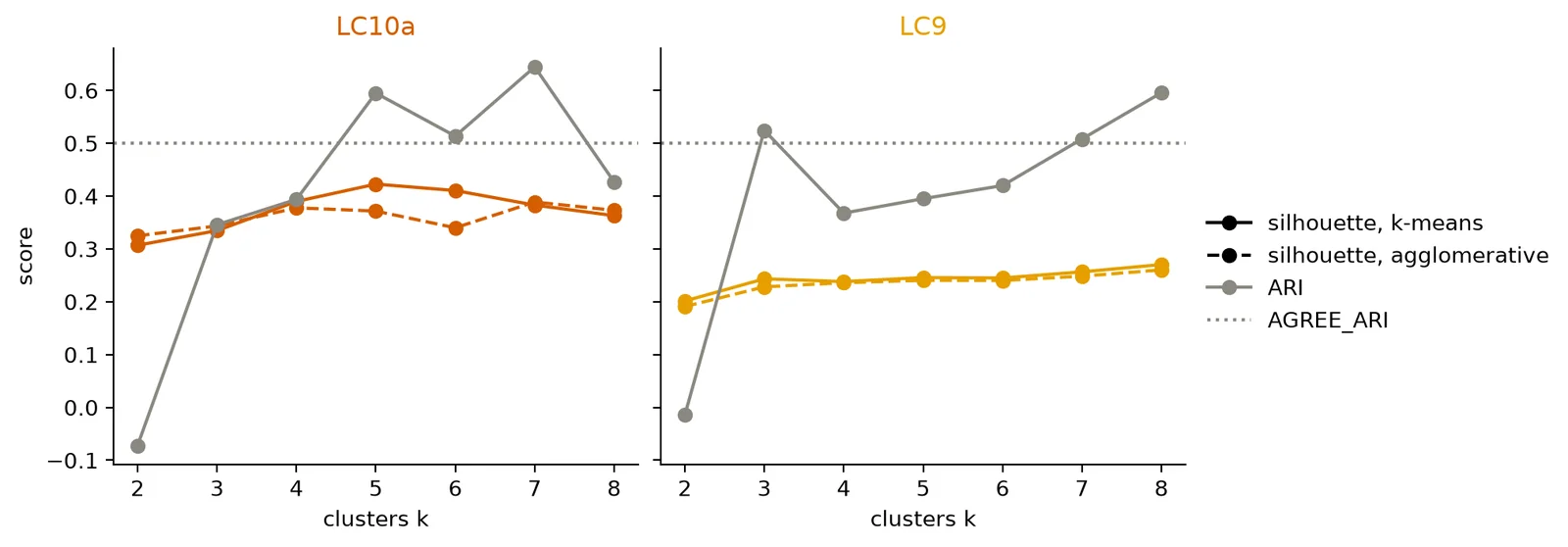
The curves show where the methods agree (the ARI against the dotted line at AGREE_ARI) and how well each clustering separates the cells (the silhouettes).

_fig, _axes = plt.subplots(1, len(TYPES), figsize=(10, 3.4), sharey=True)
for _ax, _t in zip(_axes, TYPES, strict=True):
    _s = scores.filter(pl.col("type") == _t)
    _ax.plot(
        _s["k"], _s["silhouette_kmeans"], color=TYPE_COLORS[_t], marker="o"
    )
    _ax.plot(
        _s["k"],
        _s["silhouette_agglomerative"],
        color=TYPE_COLORS[_t],
        linestyle="--",
        marker="o",
    )
    _ax.plot(_s["k"], _s["ari"], color=CONTEXT_COLOR, marker="o")
    _ax.axhline(AGREE_ARI, color=CONTEXT_COLOR, linestyle=":")
    _ax.set_title(_t, color=TYPE_COLORS[_t])
    _ax.set_xlabel("clusters k")
_axes[0].set_ylabel("score")
_fig.legend(
    handles=[
        Line2D([], [], color="k", marker="o", label="silhouette, k-means"),
        Line2D(
            [],
            [],
            color="k",
            linestyle="--",
            marker="o",
            label="silhouette, agglomerative",
        ),
        Line2D([], [], color=CONTEXT_COLOR, marker="o", label="ARI"),
        Line2D(
            [],
            [],
            color=CONTEXT_COLOR,
            linestyle=":",
            label="AGREE_ARI",
        ),
    ],
    loc="outside right",
)
_fig

chosen_k picks the number of clusters to examine: the \(k\) with the best k-means silhouette among those where the ARI reaches agree_ari, or among all of them when none does.

def chosen_k(scores: pl.DataFrame, *, agree_ari: float = AGREE_ARI) -> int:
    """The k with the largest silhouette_kmeans among the rows of
    scores with ari at or above agree_ari, or among all rows when none
    reaches it.

    scores is DataFrame[k, silhouette_kmeans, ari, ...], one row per k.
    """
    agreed = scores.filter(pl.col("ari") >= agree_ari)
    pool = agreed if agreed.height else scores
    return int(pool.sort("silhouette_kmeans")["k"][-1])

chosen_k(
    pl.DataFrame(
        {
            "k": [2, 3, 4],
            "silhouette_kmeans": [0.2, 0.5, 0.4],
            "ari": [0.9, 0.3, 0.8],
        }
    )
)

4

The chosen \(k\) of each type, whether any \(k\) reaches AGREE_ARI, the ARI there, and the sizes of the k-means clusters:

_rows = []
labels = {}
for _t in TYPES:
    _s = scores.filter(pl.col("type") == _t)
    _k = chosen_k(_s)
    labels[_t] = kmeans_labels(profiles[_t].matrix, _k)
    _rows.append(
        {
            "type": _t,
            "k": _k,
            "some k agrees": bool((_s["ari"] >= AGREE_ARI).any()),
            "ARI at k": _s.filter(pl.col("k") == _k)["ari"].item(),
            "cluster sizes": ", ".join(
                str(_n) for _n in np.bincount(labels[_t])
            ),
        }
    )
chosen = pl.DataFrame(_rows)
chosen

shape: (2, 5)

type	k	some k agrees	ARI at k	cluster sizes
str	i64	bool	f64	str
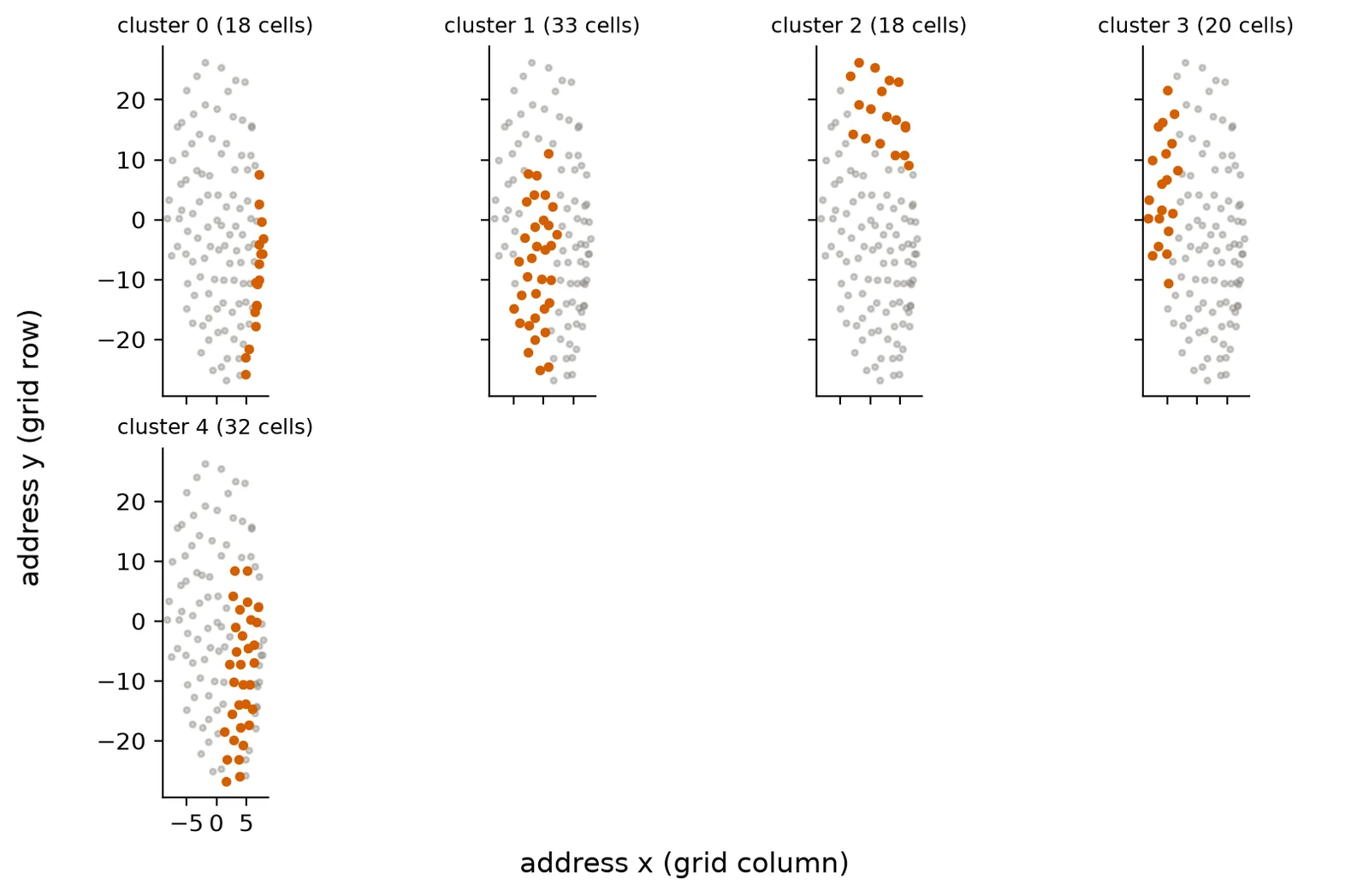
"LC10a"	5	true	0.594904	"18, 33, 18, 20, 32"
"LC9"	8	true	0.595614	"6, 15, 24, 11, 7, 11, 14, 4"

Retinotopic address

LC cells are not in column_assignment, but many of their presynaptic cells are. For an LC cell \(i\), let \(C_i\) be its presynaptic cells that have a column \((x_c, y_c)\). The address of \(i\) is the mean of their columns, weighted by their connections onto it,

\[ (x_i, y_i) = \frac{\sum_{c \in C_i} w(c \to i)\,(x_c, y_c)} {\sum_{c \in C_i} w(c \to i)}. \]

A cell with no columnar input has no address. retinotopic_addresses returns the address of each cell and the number of its columnar inputs. On three connections onto one cell:

def retinotopic_addresses(
    inputs: pl.DataFrame, columns: pl.DataFrame
) -> pl.DataFrame:
    """The weighted mean column of the presynaptic cells of each cell.

    inputs is DataFrame[pre_pt_root_id, post_pt_root_id, weight] and
    columns is DataFrame[root_id, x, y].
    DataFrame[cell, x, y, n_columnar]: n_columnar counts the columnar
    cells that connect to it; a cell with none has no row.
    """
    return (
        inputs.join(
            columns.select("root_id", "x", "y"),
            left_on="pre_pt_root_id",
            right_on="root_id",
        )
        .group_by("post_pt_root_id")
        .agg(
            x=(pl.col("weight") * pl.col("x")).sum() / pl.col("weight").sum(),
            y=(pl.col("weight") * pl.col("y")).sum() / pl.col("weight").sum(),
            n_columnar=pl.len(),
        )
        .rename({"post_pt_root_id": "cell"})
        .sort("cell")
    )

retinotopic_addresses(
    pl.DataFrame(
        {
            "pre_pt_root_id": [1, 2, 3],
            "post_pt_root_id": [9, 9, 9],
            "weight": [3, 1, 5],
        }
    ),
    pl.DataFrame({"root_id": [1, 2], "x": [0, 4], "y": [2, 2]}),
)

shape: (1, 4)

cell	x	y	n_columnar
i64	f64	f64	u32
9	1.0	2.0	2

The addresses of the real cells, and how many cells have one:

addresses = {
    _t: retinotopic_addresses(
        inputs.filter(pl.col("post_pt_root_id").is_in(cells[_t])), columns
    )
    for _t in TYPES
}
pl.DataFrame(
    {
        "type": list(TYPES),
        "cells": [len(cells[_t]) for _t in TYPES],
        "cells with an address": [addresses[_t].height for _t in TYPES],
        "median columnar inputs": [
            addresses[_t]["n_columnar"].median() for _t in TYPES
        ],
    }
)

shape: (2, 4)

type	cells	cells with an address	median columnar inputs
str	i64	i64	f64
"LC10a"	121	121	15.0
"LC9"	92	92	16.0

Each coordinate is split into N_REGION_BINS bins of equal size within the type, bin 0 holding the lowest values. The \((x, y)\) grid is retinotopic, but naming its axes frontal, lateral, or posterior needs a map of the grid onto the visual field, so the bins are named by grid position. coordinate_bins returns the bin of each value and leaves a missing value missing. On six values and three bins:

def coordinate_bins(
    values: pl.Series, n_bins: int = N_REGION_BINS
) -> pl.Series:
    """The bin of each value along one coordinate: 0 for the lowest
    n / n_bins values, up to n_bins - 1 for the highest.

    Ties are broken by position, so the bins have equal sizes (to
    within one value); a null stays null.
    """
    ranked = values.rank(method="ordinal") - 1
    return (ranked * n_bins // values.drop_nulls().len()).alias(values.name)

coordinate_bins(pl.Series("y", [5.0, 1.0, 3.0, 2.0, 6.0, 4.0]))

shape: (6,)

y
u32
2
0
1
0
2
1

Clusters on the grid

Each panel shows the cells of one cluster in color on the addresses of all the cells of the type (gray), for the chosen \(k\) of each type.

placed = {}
for _t in TYPES:
    _frame = pl.DataFrame({"cell": cells[_t], "cluster": labels[_t]}).join(
        addresses[_t], on="cell", how="left"
    )
    placed[_t] = _frame.with_columns(
        x_bin=coordinate_bins(_frame["x"]),
        y_bin=coordinate_bins(_frame["y"]),
    )
placed[TYPES[0]]

shape: (121, 7)

cell	cluster	x	y	n_columnar	x_bin	y_bin
i64	i32	f64	f64	u32	u32	u32
720575940606099586	4	3.227273	-5.159091	17	1	1
720575940607548683	3	-8.2	0.2	7	0	1
720575940610131093	4	6.185185	-6.981481	17	2	1
720575940610501093	3	-5.130435	6.695652	15	0	2
720575940611275310	1	-4.068966	-7.0	18	0	1
…	…	…	…	…	…	…
720575940645190510	4	3.875	-25.916667	11	1	0
720575940645603095	3	-6.5	-4.5	3	0	1
720575940648939897	1	1.014706	-13.882353	28	1	0
720575940650450934	0	7.117647	2.588235	7	2	1
720575940658842753	1	-2.716981	-9.490566	22	0	1

def cluster_grid_figure(
    placed: pl.DataFrame, color: str, *, ncols: int = 4
) -> Figure:
    """One panel per cluster, with the cells of the cluster in color on
    the addresses of all the cells in gray.

    placed is DataFrame[cluster, x, y, ...] with clusters 0 to k - 1;
    cells with no address are left out.
    """
    drawn = placed.drop_nulls("x")
    n_clusters = int(placed["cluster"].max()) + 1
    nrows = -(-n_clusters // ncols)
    fig, axes = plt.subplots(
        nrows,
        ncols,
        figsize=(2 * ncols, 2.6 * nrows),
        sharex=True,
        sharey=True,
        squeeze=False,
    )
    for cluster, ax in enumerate(axes.flat):
        if cluster >= n_clusters:
            ax.set_axis_off()
            continue
        own = drawn.filter(pl.col("cluster") == cluster)
        ax.scatter(drawn["x"], drawn["y"], s=6, color=CONTEXT_COLOR, alpha=0.4)
        ax.scatter(own["x"], own["y"], s=10, color=color)
        ax.set_title(f"cluster {cluster} ({own.height} cells)", fontsize=9)
        ax.set_aspect("equal")
        ax.locator_params(axis="x", nbins=3)
    fig.supxlabel("address x (grid column)")
    fig.supylabel("address y (grid row)")
    return fig

_figures = {
    _t: cluster_grid_figure(placed[_t], TYPE_COLORS[_t]) for _t in TYPES
}
mo.vstack(
    [_item for _t in TYPES for _item in (mo.md(f"**{_t}**"), _figures[_t])]
)

LC10aLC9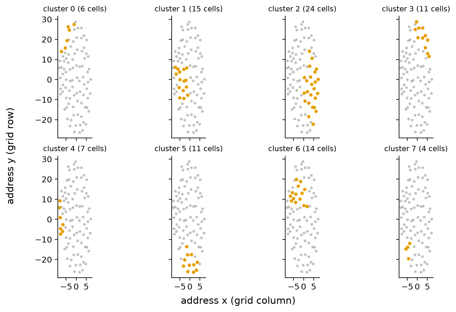

modal_bins measures how much a cluster sits in one bin: for each cluster and each coordinate, the bin that holds most of the cluster's cells that have an address, and the share of them it holds.

def modal_bins(placed: pl.DataFrame) -> pl.DataFrame:
    """The most common bin of each cluster along each coordinate.

    placed is DataFrame[cluster, x_bin, y_bin, ...]; cells with a null
    bin are left out.
    DataFrame[cluster, coordinate, bin, cells, with_bin, share]: cells
    is the number of cells of the cluster in that bin, with_bin the
    number of its cells that have a bin, share their ratio, and a tie
    goes to the lower bin.
    """
    frames = []
    for coordinate in ("x", "y"):
        counts = (
            placed.drop_nulls(f"{coordinate}_bin")
            .group_by("cluster", f"{coordinate}_bin")
            .len()
            .rename({f"{coordinate}_bin": "bin", "len": "cells"})
        )
        frames.append(
            counts.sort("cells", "bin", descending=[True, False])
            .group_by("cluster")
            .agg(
                pl.col("bin").first(),
                pl.col("cells").first(),
                with_bin=pl.col("cells").sum(),
                share=pl.col("cells").first() / pl.col("cells").sum(),
            )
            .with_columns(coordinate=pl.lit(coordinate))
        )
    return (
        pl.concat(frames)
        .select("cluster", "coordinate", "bin", "cells", "with_bin", "share")
        .sort("cluster", "coordinate")
    )

modal_bins(
    pl.DataFrame(
        {
            "cluster": [0, 0, 0, 1, 1],
            "x_bin": [0, 0, 1, 2, 2],
            "y_bin": [0, 1, 2, 2, 1],
        }
    )
)

shape: (4, 6)

cluster	coordinate	bin	cells	with_bin	share
i64	str	i64	u32	u32	f64
0	"x"	0	2	3	0.666667
0	"y"	0	1	3	0.333333
1	"x"	2	2	2	1.0
1	"y"	1	1	2	0.5

modal = pl.concat(
    [modal_bins(placed[_t]).with_columns(type=pl.lit(_t)) for _t in TYPES]
).select("type", pl.exclude("type"))
modal

shape: (26, 7)

type	cluster	coordinate	bin	cells	with_bin	share
str	i32	str	u32	u32	u32	f64
"LC10a"	0	"x"	2	18	18	1.0
"LC10a"	0	"y"	0	10	18	0.555556
"LC10a"	1	"x"	0	17	33	0.515152
"LC10a"	1	"y"	0	14	33	0.424242
"LC10a"	2	"x"	1	7	18	0.388889
…	…	…	…	…	…	…
"LC9"	5	"y"	0	11	11	1.0
"LC9"	6	"x"	0	7	14	0.5
"LC9"	6	"y"	2	10	14	0.714286
"LC9"	7	"x"	0	4	4	1.0
"LC9"	7	"y"	0	4	4	1.0

Partner types of the clusters

Clusters can differ in which partner cells they reach while reaching the same partner types. cluster_type_profile separates the two: it takes the mean profile of each cluster and adds it up over the partners of each type. On the profiles of the earlier demo, two cells in two clusters, where partners 10 and 11 are of type A and partner 12 of type B:

def cluster_type_profile(
    profiles: Profiles, labels: np.ndarray, partner_types: dict[int, str]
) -> pl.DataFrame:
    """The mean output of each cluster onto the partners of each type.

    labels gives the cluster of each cell of profiles, and
    partner_types maps a partner's root id to its type.
    DataFrame[cluster, partner_type, share]: share is the mean over the
    cells of the cluster of the profile summed over that type.
    """
    types = np.array([partner_types[p] for p in profiles.partners])
    rows = []
    for cluster in np.unique(labels):
        mean_profile = profiles.matrix[labels == cluster].mean(axis=0)
        rows += [
            {
                "cluster": int(cluster),
                "partner_type": name,
                "share": float(mean_profile[types == name].sum()),
            }
            for name in np.unique(types)
        ]
    return pl.DataFrame(rows)

cluster_type_profile(
    Profiles(
        cells=[1, 2],
        partners=[10, 11, 12],
        matrix=np.array([[0.75, 0.25, 0.0], [0.0, 0.5, 0.5]]),
    ),
    np.array([0, 1]),
    {10: "A", 11: "A", 12: "B"},
)

shape: (4, 3)

cluster	partner_type	share
i64	str	f64
0	"A"	1.0
0	"B"	0.0
1	"A"	0.5
1	"B"	0.5

The heatmaps show the types that take the largest share of any cluster, with the share of each cluster in each type.

type_profiles = {}
for _t in TYPES:
    _partner_types = dict(
        partners.filter(pl.col("type") == _t)
        .select("partner", "partner_type")
        .iter_rows()
    )
    type_profiles[_t] = cluster_type_profile(
        profiles[_t], labels[_t], _partner_types
    )
_charts = []
for _t in TYPES:
    _top = (
        type_profiles[_t]
        .group_by("partner_type")
        .agg(pl.col("share").max())
        .sort("share", descending=True)
        .head(10)["partner_type"]
        .to_list()
    )
    _charts.append(
        alt.Chart(
            type_profiles[_t].filter(pl.col("partner_type").is_in(_top))
        )
        .mark_rect()
        .encode(
            x=alt.X("cluster:O", title=f"{_t} cluster"),
            y=alt.Y("partner_type:N", sort=_top, title=None),
            color=alt.Color(
                "share:Q",
                scale=alt.Scale(scheme="greys", domain=[0, 0.5]),
                legend=alt.Legend(format="%", title="share of output"),
            ),
            tooltip=[
                "cluster:O",
                "partner_type:N",
                alt.Tooltip("share:Q", format=".1%"),
            ],
        )
        .properties(width=160, height=170)
    )
alt.hconcat(*_charts)

bin_name says a bin in words, for the sentences that describe where a cluster sits:

def bin_name(bin_: int, n_bins: int = N_REGION_BINS) -> str:
    """The bin as a word: lowest, highest, or middle.

    Raises ValueError for a bin outside 0 to n_bins - 1.
    """
    if not 0 <= bin_ < n_bins:
        msg = f"bin {bin_} is outside 0 to {n_bins - 1}"
        raise ValueError(msg)
    if bin_ == 0:
        return "lowest"
    if bin_ == n_bins - 1:
        return "highest"
    return "middle"

[bin_name(_b) for _b in range(N_REGION_BINS)]

• 0: 'lowest'
• 1: 'middle'
• 2: 'highest'

Discussion

Expectation 1: The two methods agree on some k for every type. The ARI reaches AGREE_ARI at LC10a (k = 5, 6, 7) and LC9 (k = 3, 7, 8) (Clusters that two methods agree on). At the chosen k the k-means silhouette is LC10a 0.42 and LC9 0.27 and the ARI is LC10a 0.59 and LC9 0.60. For LC9 the chosen k is the largest in K_GRID, so a better k may lie beyond it.

Expectation 2: Some clusters of every type sit in one bin. At least PURE_SHARE of the cells are in one bin of \(x\) or \(y\) in LC10a 3 of 5 and LC9 5 of 8 clusters, where a cluster that ignored position would hold about 33% of its cells in each bin (Clusters on the grid). The clusters that do:

• LC10a cluster 0: 18 of 18 cells in the highest x bin
• LC10a cluster 2: 18 of 18 cells in the highest y bin
• LC10a cluster 3: 20 of 20 cells in the lowest x bin
• LC9 cluster 0: 6 of 6 cells in the highest y bin
• LC9 cluster 3: 11 of 11 cells in the highest y bin
• LC9 cluster 4: 7 of 7 cells in the lowest x bin
• LC9 cluster 5: 11 of 11 cells in the lowest y bin
• LC9 cluster 7: 4 of 4 cells in the lowest x bin
• LC9 cluster 7: 4 of 4 cells in the lowest y bin

The heaviest partner type of each cluster. LC10a: cluster 0 CB2070 (23%), cluster 1 TuTuAa (12%), cluster 2 TuTuAa (15%), cluster 3 AOTUv3B_P01 (19%), and cluster 4 TuTuAa (13%); LC9: cluster 0 PVLP004 (26%), cluster 1 PVLP004 (25%), cluster 2 PVLP004 (31%), cluster 3 PVLP004 (30%), cluster 4 PVLP004 (34%), cluster 5 PVLP004 (32%), cluster 6 PVLP004 (24%), and cluster 7 PVLP004 (28%). The heaviest type is the same in every cluster of LC9. The heatmaps show how the rest of each cluster's output is shared (Partner types of the clusters).

Skeptic's case. Clustering on partner identity recovers retinotopic neighborhoods whenever the partners are themselves retinotopic, as the targets of an LC type in the AOTu are expected to be. The clusters may be patches cut from one continuous population, and low silhouettes or partial agreement between the methods fit that. A partner type that covers only part of the visual field looks specific to a cluster even in a continuum.

Conclusion. The clusters of LC10a and LC9 occupy parts of the grid, so output connectivity carries retinotopic position there. Whether the groups are discrete or patches of one continuum, the claim that matters for pairing sub-populations, is not decided here (Open questions).

Limitations

A profile counts only the output onto the strong partners that are proofread neurons and not LC cells, so it leaves out the weak and the unproofread output of a cell, and a cell with no such partner would have a profile of zeros (there are none among these cells). The address is the mean column of the columnar inputs of a cell, so it places a cell by the middle of its inputs, not by the extent of its dendrite, and a cell with no columnar input would have no address and be left out of the grid figures (there are none among these cells). The bins are equal in size within a type, so they say where a cell is relative to the others of its type, not where it is in the visual field. The clusters come from one k-means start, RANDOM_STATE, and are not compared across seeds.

Open questions

1. Is a type a continuum, with no step in its profiles between clusters? Test: the cosine similarity of the profiles of two cells against the distance between their addresses, split by whether the cells share a cluster. Refuted if cells of one cluster are more similar than cells of different clusters at the same distance.
2. Are the partner types that belong to one cluster restricted to a region of the grid? Test: the addresses of the cells that contact such a type against the addresses of all the cells of the type. Refuted if, at the same address, the cells of the cluster contact the type and their neighbors in other clusters do not.
3. Do the whole-type overlaps of lc_pathways understate the convergence of cells that view the same region? Test: the overlap of strong partners between cells of two types with the same address bins against cells with different bins. Refuted if the two give the same overlap.

Terms

• address: the mean visual-column position \((x, y)\) of the columnar cells that connect to an LC cell, weighted by weight.
• adjusted Rand index (ARI): how much two labelings of the same cells agree, 1 for the same grouping and 0 for the agreement of chance.
• agglomerative clustering: clustering that starts with every cell alone and merges the two closest clusters until \(k\) remain.
• bin: one of N_REGION_BINS equal-size ranges of an address coordinate within a type.
• k-means: clustering that places \(k\) centers to minimize the squared distance of each profile to its nearest center.
• lateral partner: an LC cell that receives a connection from a cell of the type; it is not a strong partner here.
• output profile: the weights of a cell onto the strong partners of its type, divided by their total.
• partner: a postsynaptic segment of a connection from some cell of a type, either a proofread neuron or an unproofread fragment. LC cells count.
• proofread neuron: a segment that people have proofread and joined into a neuron (proofread_ids).
• silhouette: the mean over cells of how much closer a cell is to its own cluster than to the nearest other cluster, from \(-1\) to 1.
• strength \(s(T \to j)\): the weight of the heaviest single connection from a cell of the type \(T\) onto the partner \(j\).
• strong partner: a proofread partner that is not an LC cell and has a strength of at least STRONG_SYN.
• weight \(w(i \to j)\): the number of synapses in the connection from \(i\) to \(j\).