LC output strength: definitions
Introduction
Question
What other ways could a partner's strength be defined, and how do they differ?
Background
lc_output_strength gives each partner of an LC type one strength,
the weight of the heaviest single connection onto it from one cell
of the type,
and takes the partners at or above STRONG_SYN as strong.
Here that strength is \(s_{\mathrm{max}}\), because there are three.
STRONG_SYN is Dr. Chiappe's suggestion.
Dr. Chiappe also suggested taking the cutoff wherever the
distribution of strengths shows a kink.
Nothing here ranks the definitions; it describes how they differ.
Reading a cutoff from the distribution
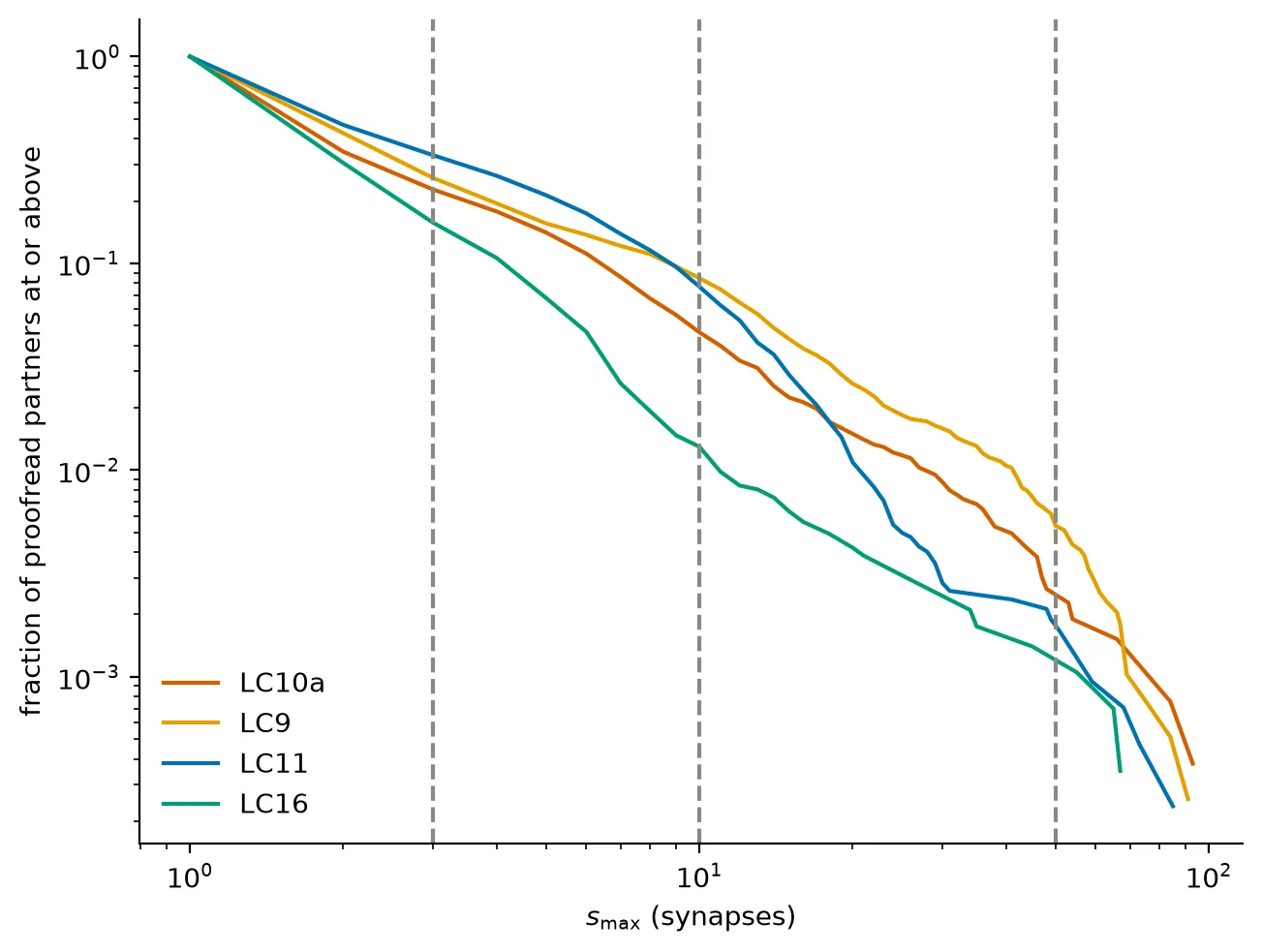
Most connections carry one or two synapses and a few carry dozens, so strengths have a heavy tail. A heavy tail is easiest to read on its complementary cumulative distribution function (CCDF), \(F(m)\), drawn on log-log axes,
A single skewed distribution gives a smooth curve with no natural cutoff; a bend would suggest a distinct group of strong partners. Between two marks \(m_a < m_b\) the local slope is
A power law has constant \(\beta\), and a weak bulk that falls off faster than the tail shows as \(\beta\) becoming less negative past the bend.
Three strengths
A strength summarizes the weights of a partner's connections from
one type.
\(s_{\mathrm{max}}\) looks at one connection, so a partner that many
cells connect to weakly never reaches a high \(s_{\mathrm{max}}\).
This notebook adds two strengths that add up the cells of the type
(defined below):
\(s_{\mathrm{sum}}\), the number of synapses all cells of the type
send to the partner,
and \(s_{\mathrm{sum,filtered}}\), the same sum over the strong
connections only, those of at least STRONG_SYN synapses.
A partner is strong by a strength when that strength is at or above
STRONG_SYN.
The release paper reports the input of a group of neurons to a
neuron as a sum:
We found that 15 different descending neurons each receive more than 200 synapses from the OCG01 neurons.
— Dorkenwald et al. 2024, p. 135 · PDF p. 135 · 10.1038/s41586-024-07558-y
It sets no cutoff for such a sum, and this notebook looks for none for \(s_{\mathrm{sum,filtered}}\): the aim is to see how the strengths are distributed. A sum is never smaller than a maximum, so \(s_{\mathrm{sum}} \ge s_{\mathrm{max}}\), and every partner strong by \(s_{\mathrm{max}}\) is strong by \(s_{\mathrm{sum}}\). A partner with no strong connection has \(s_{\mathrm{sum,filtered}} = 0\), and one with a strong connection has \(s_{\mathrm{sum,filtered}} \ge s_{\mathrm{max}}\), so the partners with a nonzero \(s_{\mathrm{sum,filtered}}\) are exactly the partners strong by \(s_{\mathrm{max}}\), ranked by how much their strong connections carry.
Expectations
For each type, whichever partners count (proofread neurons only or fragments as well, lateral partners or not):
- Under \(s_{\mathrm{max}}\) the slope of the CCDF changes near 10 synapses: the chords flatten across it, and the knot of the bend fit and the start of the power-law fit lie there.
- Under \(s_{\mathrm{sum}}\) they lie at a higher strength, because a sum is larger than a maximum.
Load data
The analysis reads four tables. census gives each cell's type.
sides says which hemisphere a cell is in,
and proofread_ids lists the proofread neurons.
connections has one row per connection, a pair of cells with at
least one synapse, as in the name of Codex's
connections_princeton_no_threshold table, with its weight and
the type of its presynaptic cell.
The table of every proofread neuron's connections has about a
hundred million rows, so this notebook loads only the connections
that start at the cells it scores.
| root_id | primary_type |
|---|---|
| i64 | str |
| 720575940599457990 | "T4b" |
| 720575940599763910 | "T5b" |
| 720575940600623020 | "Dm3q" |
| 720575940602564320 | "KCg-m" |
| 720575940602720940 | "JO-CA" |
| … | … |
| 720575940661275009 | "KCab-p" |
| 720575940661281409 | "L4" |
| 720575940661285249 | "LPC2" |
| 720575940661304449 | "Lawf1" |
| 720575940661333889 | "CB2303" |
| root_id | side |
|---|---|
| i64 | str |
| 720575940596125868 | "right" |
| 720575940597856265 | "right" |
| 720575940597944841 | "right" |
| 720575940598267657 | "right" |
| 720575940599333574 | "right" |
| … | … |
| 720575940661323905 | "left" |
| 720575940661325697 | "left" |
| 720575940661327745 | "right" |
| 720575940661336193 | "left" |
| 720575940661339777 | "right" |
| root_id |
|---|
| i64 |
| 720575940599457990 |
| 720575940599763910 |
| 720575940600623020 |
| 720575940602309600 |
| 720575940602564320 |
| … |
| 720575940661275009 |
| 720575940661281409 |
| 720575940661285249 |
| 720575940661304449 |
| 720575940661333889 |
The four types of interest are restricted to the right hemisphere.
cells = cells_of_types(census, sides, TYPES_OF_INTEREST)
pl.DataFrame(
    {
        "type": list(TYPES_OF_INTEREST),
        "right-hemisphere cells": [
            len(cells[_t]) for _t in TYPES_OF_INTEREST
        ],
    }
)
| type | right-hemisphere cells |
|---|---|
| str | i64 |
| "LC10a" | 121 |
| "LC9" | 92 |
| "LC11" | 61 |
| "LC16" | 74 |
connections is filtered while it loads to the connections whose
presynaptic cell is one of those cells.
with_pre_type (from helpers) labels each
with the type of its presynaptic cell, in the column pre_type.
A strength is taken over the cells of one type,
so the label says which connections belong together:
_scored = [_id for _ids in cells.values() for _id in _ids]
connections = with_pre_type(load_connections_of(_scored), cells)
connections
| pre_pt_root_id | post_pt_root_id | weight | pre_type |
|---|---|---|---|
| i64 | i64 | i64 | str |
| 720575940603578848 | 720575940381391499 | 1 | "LC11" |
| 720575940603578848 | 720575940381415307 | 1 | "LC11" |
| 720575940603578848 | 720575940381421195 | 1 | "LC11" |
| 720575940603578848 | 720575940381425291 | 1 | "LC11" |
| 720575940603578848 | 720575940381433227 | 1 | "LC11" |
| … | … | … | … |
| 720575940659229057 | 720575940649865718 | 1 | "LC11" |
| 720575940659229057 | 720575940650149753 | 2 | "LC11" |
| 720575940659229057 | 720575940651404278 | 2 | "LC11" |
| 720575940659229057 | 720575940653346038 | 2 | "LC11" |
| 720575940659229057 | 720575940661134465 | 1 | "LC11" |
The three strengths
For a type \(T\) and a partner \(j\),
\(s_{\mathrm{max}}(j)\) is the largest weight \(w(i \to j)\) onto \(j\)
from one cell
\(i\) of \(T\), where a weight is the number of synapses in one
connection.
\(s_{\mathrm{sum}}\) adds the weights of all of them,
and \(s_{\mathrm{sum,filtered}}\) adds only those at or above
STRONG_SYN:
strengths_to_partners returns \(s_{\mathrm{sum}}\) as synapses,
and strong_connection_sums returns \(s_{\mathrm{sum,filtered}}\)
for the partners that have a strong connection;
the others get 0.
A partner that two cells connect to with weights 6 and 5
has \(s_{\mathrm{max}} = 6\) and \(s_{\mathrm{sum}} = 11\) but
\(s_{\mathrm{sum,filtered}} =
0\),
so at STRONG_SYN it is strong by \(s_{\mathrm{sum}}\) and not
by \(s_{\mathrm{max}}\).
A partner with weights 11 and 4 has \(s_{\mathrm{max}} = 11\),
\(s_{\mathrm{sum}} = 15\) and \(s_{\mathrm{sum,filtered}} = 11\):
def strong_connection_sums(
    connections: pl.DataFrame,
    *,
    by: str = "pre_type",
    cutoff: int = STRONG_SYN,
) -> pl.DataFrame:
    """The summed weight of the strong connections onto each partner
    that has one, a strong connection having a weight of at least
    cutoff.

    by labels the presynaptic cells, as in strengths_to_partners.
    DataFrame[by, partner, s_sum_filtered]; a partner with no strong
    connection has no row.
    """
    return (
        connections.drop_nulls(by)
        .filter(pl.col("weight") >= cutoff)
        .group_by(by, "post_pt_root_id")
        .agg(s_sum_filtered=pl.col("weight").sum())
        .rename({"post_pt_root_id": "partner"})
    )
_two = pl.DataFrame(
    {
        "pre_pt_root_id": ["t1", "t2", "t1", "t2"],
        "post_pt_root_id": ["j", "j", "k", "k"],
        "weight": [6, 5, 11, 4],
        "pre_type": ["T", "T", "T", "T"],
    }
)
strengths_to_partners(_two).join(
    strong_connection_sums(_two),
    on=["pre_type", "partner"],
    how="left",
).with_columns(pl.col("s_sum_filtered").fill_null(0))
| pre_type | partner | s | synapses | cells | s_sum_filtered |
|---|---|---|---|---|---|
| str | str | i64 | i64 | u32 | i64 |
| "T" | "j" | 6 | 11 | 2 | 0 |
| "T" | "k" | 11 | 15 | 2 | 11 |
strengths_to_partners_with_cell_fraction and label_partners
build the table of lc_output_strength for the partners of the
four types.
Here s becomes s_max, synapses becomes s_sum,
strong_connection_sums gives
s_sum_filtered, which is joined on,
and group says which strengths call the partner strong:
partners = (
    label_partners(
        strengths_to_partners_with_cell_fraction(connections, cells),
        census,
        proofread_ids,
    )
    .rename({"synapses": "s_sum", "s": "s_max"})
    .join(
        strong_connection_sums(connections).rename({"pre_type": "type"}),
        on=["type", "partner"],
        how="left",
    )
    .with_columns(pl.col("s_sum_filtered").fill_null(0))
    .with_columns(
        group=pl.when(pl.col("s_max") >= STRONG_SYN)
        .then(pl.lit("strong by s_max"))
        .when(pl.col("s_sum") >= STRONG_SYN)
        .then(pl.lit("strong by s_sum only"))
        .otherwise(pl.lit("weak"))
    )
)
proofread_partners = partners.filter(pl.col("proofread"))
populations = partner_populations(partners)
partners
| type | partner | s_max | s_sum | cells | cell_fraction | partner_type | proofread | lateral | s_sum_filtered | group |
|---|---|---|---|---|---|---|---|---|---|---|
| str | i64 | i64 | i64 | u32 | f64 | str | bool | bool | i64 | str |
| "LC10a" | 720575940379710175 | 1 | 1 | 1 | 0.008264 | "unproofread fragment" | false | false | 0 | "weak" |
| "LC10a" | 720575940379714527 | 1 | 1 | 1 | 0.008264 | "unproofread fragment" | false | false | 0 | "weak" |
| "LC10a" | 720575940379724716 | 1 | 1 | 1 | 0.008264 | "unproofread fragment" | false | false | 0 | "weak" |
| "LC10a" | 720575940379730143 | 1 | 1 | 1 | 0.008264 | "unproofread fragment" | false | false | 0 | "weak" |
| "LC10a" | 720575940379737004 | 1 | 1 | 1 | 0.008264 | "unproofread fragment" | false | false | 0 | "weak" |
| … | … | … | … | … | … | … | … | … | … | … |
| "LC9" | 720575940660758401 | 1 | 1 | 1 | 0.01087 | "Li08" | true | false | 0 | "weak" |
| "LC9" | 720575940661134465 | 2 | 4 | 3 | 0.032609 | "Li06" | true | false | 0 | "weak" |
| "LC9" | 720575940661244033 | 2 | 2 | 1 | 0.01087 | "TmY15" | true | false | 0 | "weak" |
| "LC9" | 720575940661318017 | 2 | 5 | 3 | 0.032609 | "LLPC3" | true | false | 0 | "weak" |
| "LC9" | 720575940661327745 | 1 | 1 | 1 | 0.01087 | "LTe09" | true | false | 0 | "weak" |
Strengths of the proofread partners
From here to the strong-set figure, partners are the proofread neurons. The table gives the scale of the data: how many partners each type has, how strong the typical one is, and how many partners each strength calls strong. The three last columns count the unproofread fragments that \(s_{\mathrm{max}}\) would add to the strong set, the proofread partners that are LC cells, and how many of those are strong.
partner_counts = partners.group_by("type", maintain_order=True).agg(
    (pl.col("proofread").sum()).alias("proofread partners"),
    pl.col("s_sum")
    .filter(pl.col("proofread"))
    .median()
    .alias("median s_sum"),
    pl.col("s_max")
    .filter(pl.col("proofread"))
    .median()
    .alias("median s_max"),
    pl.col("s_sum").filter(pl.col("proofread")).max().alias("max s_sum"),
    pl.col("s_max").filter(pl.col("proofread")).max().alias("max s_max"),
    ((pl.col("group") == "strong by s_max") & pl.col("proofread"))
    .sum()
    .alias("strong by s_max"),
    ((pl.col("group") == "strong by s_sum only") & pl.col("proofread"))
    .sum()
    .alias("strong by s_sum only"),
    ((pl.col("group") == "strong by s_max") & ~pl.col("proofread"))
    .sum()
    .alias("strong fragments (s)"),
    (pl.col("lateral") & pl.col("proofread"))
    .sum()
    .alias("proofread LC partners"),
    (
        (pl.col("group") == "strong by s_max")
        & pl.col("lateral")
        & pl.col("proofread")
    )
    .sum()
    .alias("strong LC partners (s)"),
)
partner_counts
| type | proofread partners | median s_sum | median s_max | max s_sum | max s_max | strong by s_max | strong by s_sum only | strong fragments (s) | proofread LC partners | strong LC partners (s) |
|---|---|---|---|---|---|---|---|---|---|---|
| str | u32 | f64 | f64 | i64 | i64 | u32 | u32 | u32 | u32 | u32 |
| "LC10a" | 2634 | 1.0 | 1.0 | 5172 | 93 | 122 | 383 | 2 | 876 | 37 |
| "LC11" | 4231 | 2.0 | 1.0 | 2505 | 85 | 326 | 686 | 0 | 1076 | 194 |
| "LC16" | 2856 | 1.0 | 1.0 | 2614 | 67 | 37 | 263 | 0 | 714 | 2 |
| "LC9" | 3908 | 2.0 | 1.0 | 1682 | 91 | 331 | 341 | 10 | 1139 | 242 |
Each point below is a set of partners with the same pair of strengths. The strengths agree along the diagonal, where one cell connects to the partner; points above it are partners that several cells connect to. The shaded region holds the partners strong by \(s_{\mathrm{sum}}\) only, because weak connections add up. Drag a box over points to list the partners in them; hold shift and drag to draw a lasso.
_x_top = proofread_partners["s_max"].max() * 1.3
_y_top = proofread_partners["s_sum"].max() * 1.3
_widgets = {}
for _t in TYPES_OF_INTEREST:
    _p = proofread_partners.filter(pl.col("type") == _t)
    _combos = _p.group_by("s_max", "s_sum").len()
    # One figure per type so each panel has its own selection;
    # the limits are shared by hand.
    _fig, _ax = plt.subplots(figsize=(4, 3.6))
    _ax.fill(
        [0.8, STRONG_SYN, STRONG_SYN, 0.8],
        [STRONG_SYN, STRONG_SYN, _y_top, _y_top],
        color=CONTEXT_COLOR,
        alpha=0.15,
        linewidth=0,
    )
    _ax.plot(
        [0.8, _x_top], [0.8, _x_top], color=CONTEXT_COLOR, linewidth=0.8
    )
    _ax.axvline(
        STRONG_SYN, color=CONTEXT_COLOR, linestyle="--", linewidth=0.8
    )
    _ax.axhline(
        STRONG_SYN, color=CONTEXT_COLOR, linestyle="--", linewidth=0.8
    )
    _ax.scatter(
        _combos["s_max"],
        _combos["s_sum"],
        s=6 + 28 * np.log10(_combos["len"]),
        color=TYPE_COLORS[_t],
        alpha=0.55,
        linewidths=0,
    )
    _both = int((_p["group"] == "strong by s_max").sum())
    _type_only = int((_p["group"] == "strong by s_sum only").sum())
    _ax.text(
        0.96,
        0.05,
        f"{_both} strong by $s_{{\\mathrm{{max}}}}$\n"
        f"{_type_only} strong by $s_{{\\mathrm{{sum}}}}$ only",
        transform=_ax.transAxes,
        ha="right",
        va="bottom",
        fontsize=9,
    )
    _ax.set_xscale("log")
    _ax.set_yscale("log")
    _ax.set_xlim(0.8, _x_top)
    _ax.set_ylim(0.8, _y_top)
    _ax.set_title(_t, color=TYPE_COLORS[_t])
    _ax.set_xlabel(r"$s_{\mathrm{max}}$ (synapses)")
    _ax.set_ylabel(r"$s_{\mathrm{sum}}$ (synapses)")
    _widgets[_t] = mo.ui.matplotlib(_ax)
    plt.close(_fig)
scatter = mo.ui.dictionary(_widgets)
mo.vstack(
    [
        mo.hstack(
            [scatter[TYPES_OF_INTEREST[0]], scatter[TYPES_OF_INTEREST[1]]],
            justify="start",
        ),
        mo.hstack(
            [scatter[TYPES_OF_INTEREST[2]], scatter[TYPES_OF_INTEREST[3]]],
            justify="start",
        ),
    ]
)
_selected = []
for _t, _widget in scatter.items():
    _p = proofread_partners.filter(pl.col("type") == _t)
    if _widget.value:
        _mask = _widget.value.get_mask(
            _p["s_max"].to_numpy(), _p["s_sum"].to_numpy()
        )
        _selected.append(_p.filter(pl.Series(_mask)))
mo.stop(not _selected, mo.md("_No partners selected._"))
pl.concat(_selected).select(
    "type",
    "partner",
    "partner_type",
    "s_max",
    "s_sum",
    "cells",
).sort("s_sum", descending=True)
No partners selected.
The scatter says how strongly partners are connected but not by how many cells. Each dot below is one partner, placed by the percent of the type's cells that connect to it, for the partners strong by \(s_{\mathrm{max}}\) (left of each pair) and those strong by \(s_{\mathrm{sum}}\) only (right). Bars mark the medians and diamonds the medians without lateral partners. Drag a box to list the partners in it.
_rng = np.random.default_rng(0)
_strong = proofread_partners.filter(pl.col("group") != "weak")
_offset = {"strong by s_max": -0.2, "strong by s_sum only": 0.2}
# Each type gets two columns, one per group,
# with jitter so dots do not stack.
strip_points = _strong.with_columns(
    x=pl.col("type").replace_strict(
        {_t: _n for _n, _t in enumerate(TYPES_OF_INTEREST)}
    )
    + pl.col("group").replace_strict(_offset)
    + pl.Series(_rng.uniform(-0.13, 0.13, _strong.height))
)
_fig, _ax = plt.subplots(figsize=(8, 3.8))
_medians = []
for _n, _t in enumerate(TYPES_OF_INTEREST):
    for _group, _alpha in (
        ("strong by s_max", 0.8),
        ("strong by s_sum only", 0.25),
    ):
        _g = strip_points.filter(
            (pl.col("type") == _t) & (pl.col("group") == _group)
        )
        _ax.scatter(
            _g["x"],
            _g["cell_fraction"],
            s=9,
            color=TYPE_COLORS[_t],
            alpha=_alpha,
            linewidths=0,
        )
        _median = _g["cell_fraction"].median()
        _ax.hlines(
            _median,
            _n + _offset[_group] - 0.17,
            _n + _offset[_group] + 0.17,
            color="k",
            linewidth=2,
            zorder=3,
        )
        _median_no_lc = _g.filter(~pl.col("lateral"))[
            "cell_fraction"
        ].median()
        _ax.plot(
            _n + _offset[_group],
            _median_no_lc,
            "D",
            color="white",
            markeredgecolor="k",
            zorder=4,
        )
        _medians.append(
            {
                "type": _t,
                "group": _group,
                "median % of cells": _median,
                "median % of cells, no LC partners": _median_no_lc,
            }
        )
_ax.set_xticks(range(len(TYPES_OF_INTEREST)), TYPES_OF_INTEREST)
_ax.set_ylabel("% of the type's cells\nconnected to the partner")
_ax.set_ylim(0, 1.03)
_ax.yaxis.set_major_formatter(PercentFormatter(1.0))
_ax.legend(
    handles=[
        Line2D(
            [],
            [],
            marker="o",
            color="none",
            markerfacecolor=CONTEXT_COLOR,
            alpha=0.9,
            label="strong by $s_{\\mathrm{max}}$ (left of each pair)",
        ),
        Line2D(
            [],
            [],
            marker="o",
            color="none",
            markerfacecolor=CONTEXT_COLOR,
            alpha=0.35,
            label="strong by $s_{\\mathrm{sum}}$ only (right)",
        ),
    ],
    loc="lower center",
    bbox_to_anchor=(0.5, 1.0),
    ncol=2,
)
contributor_medians = pl.DataFrame(_medians)
strip = mo.ui.matplotlib(_ax)
plt.close(_fig)
strip
<marimo-matplotlib data-initial-value='{}' data-label='null' data-chart-base64='"../../assets/img/2f78dc1f2ee66a818cc3978d00662961cde62f5ca65f117bef13bd8cae732eaa.webp"' data-x-bounds='[-0.557,3.557]' data-y-bounds='[0.0,1.03]' data-axes-pixel-bounds='[93.6789357638889,36.55914409722218,795.833,352.2218888888889]' data-width='800.0' data-height='380.0' data-debounce='false' data-x-scale='"linear"' data-y-scale='"linear"'></marimo-matplotlib>
mo.stop(not strip.value, mo.md("_No partners selected._"))
_mask = strip.value.get_mask(
    strip_points["x"].to_numpy(), strip_points["cell_fraction"].to_numpy()
)
strip_points.filter(pl.Series(_mask)).select(
    "type",
    "partner",
    "partner_type",
    "group",
    "s_max",
    "s_sum",
    "cells",
    "cell_fraction",
).sort("cell_fraction", descending=True)
No partners selected.
Median percent of the type's cells connected to a partner. Strong by \(s_{\mathrm{max}}\): LC10a 27%, LC9 7%, LC11 8%, LC16 93%; without LC cells LC10a 36%, LC9 32%, LC11 71%, LC16 95%. Strong by \(s_{\mathrm{sum}}\) only: LC10a 10%, LC9 9%, LC11 10%, LC16 35%; without LC cells LC10a 11%, LC9 12%, LC11 13%, LC16 22%.
Distribution of the strengths
plot_strength_ccdf overlays the CCDFs of the types;
the dashed lines mark marks, BEND_MARKS by default.
The CCDF of \(s_{\mathrm{max}}\):
def plot_strength_ccdf(
    strengths_by_type: dict[str, ArrayLike],
    xlabel: str,
    ylabel: str,
    *,
    marks: Sequence[float] = BEND_MARKS,
) -> Figure:
    """A figure with the log-log CCDF of each type's strengths and a
    dashed vertical line at each mark."""
    fig, ax = plt.subplots()
    for type_name, strengths in strengths_by_type.items():
        curve = ccdf(strengths)
        ax.plot(curve["value"], curve["fraction"], label=type_name)
    for mark in marks:
        ax.axvline(mark, color=CONTEXT_COLOR, linestyle="--")
    ax.set_xscale("log")
    ax.set_yscale("log")
    ax.set_xlabel(xlabel)
    ax.set_ylabel(ylabel)
    ax.legend()
    return fig
s_max_by_type = strengths_by_type(proofread_partners, "s_max")
plot_strength_ccdf(
    s_max_by_type,
    r"$s_{\mathrm{max}}$ (synapses)",
    "fraction of proofread partners at or above",
)
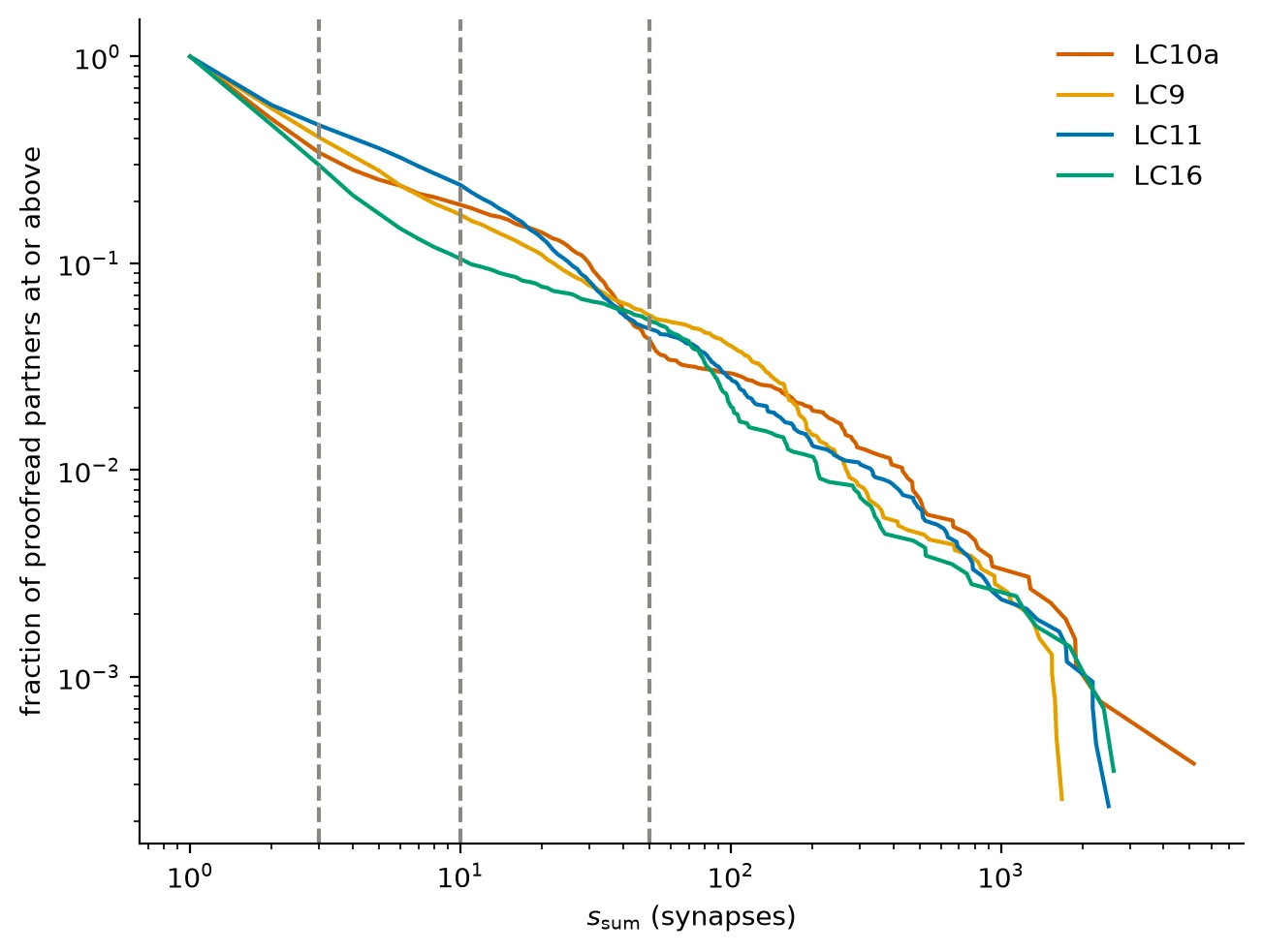
The CCDF of \(s_{\mathrm{sum}}\):
s_sum_by_type = strengths_by_type(proofread_partners, "s_sum")
plot_strength_ccdf(
    s_sum_by_type,
    r"$s_{\mathrm{sum}}$ (synapses)",
    "fraction of proofread partners at or above",
)
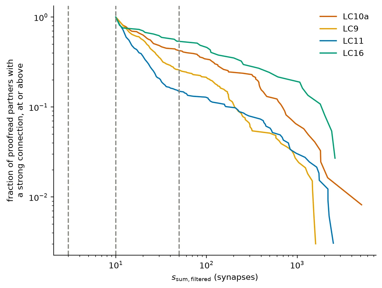
\(s_{\mathrm{sum,filtered}}\) is nonzero only for partners with a strong connection, which are the partners strong by \(s_{\mathrm{max}}\), so its CCDF covers those partners and starts at the cutoff:
s_sum_filtered_by_type = strengths_by_type(
    proofread_partners.filter(pl.col("s_sum_filtered") > 0),
    "s_sum_filtered",
)
plot_strength_ccdf(
    s_sum_filtered_by_type,
    r"$s_{\mathrm{sum,filtered}}$ (synapses)",
    "fraction of proofread partners with\n"
    "a strong connection, at or above",
)
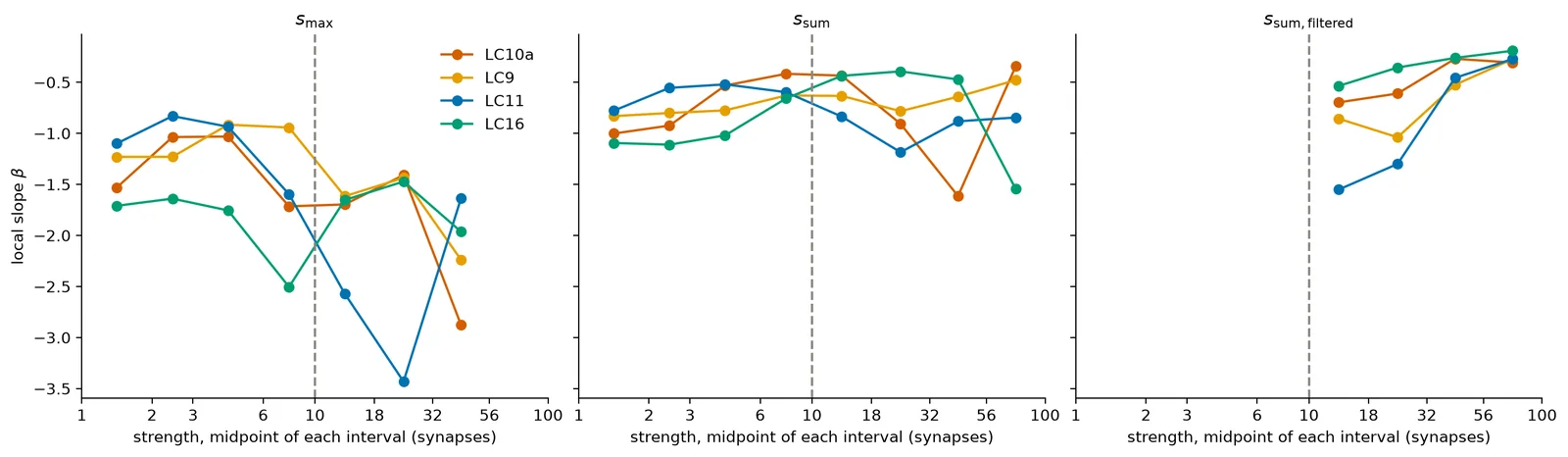
The local slope between every pair of successive SLOPE_MARKS
shows where along each curve the change happens,
and whether a sum has a bend at all.
The panel of \(s_{\mathrm{sum,filtered}}\) starts at the cutoff:
_rows = []
for _strength, _by_type in (
    ("s_max", s_max_by_type),
    ("s_sum", s_sum_by_type),
    ("s_sum_filtered", s_sum_filtered_by_type),
):
    # s_sum_filtered starts at the cutoff.
    _marks = tuple(
        _m
        for _m in SLOPE_MARKS
        if _strength != "s_sum_filtered" or _m >= STRONG_SYN
    )
    _rows += [
        local_slopes(_by_type[_t], _marks).with_columns(
            strength=pl.lit(_strength), type=pl.lit(_t)
        )
        for _t in TYPES_OF_INTEREST
    ]
slopes = pl.concat(_rows).select(
    "strength", "type", "lower", "upper", "slope"
)
slopes
| strength | type | lower | upper | slope |
|---|---|---|---|---|
| str | str | f64 | f64 | f64 |
| "s_max" | "LC10a" | 1.0 | 2.0 | -1.53015 |
| "s_max" | "LC10a" | 2.0 | 3.0 | -1.036781 |
| "s_max" | "LC10a" | 3.0 | 6.0 | -1.031655 |
| "s_max" | "LC10a" | 6.0 | 10.0 | -1.715168 |
| "s_max" | "LC10a" | 10.0 | 18.0 | -1.696804 |
| … | … | … | … | … |
| "s_sum_filtered" | "LC11" | 56.0 | 100.0 | -0.271859 |
| "s_sum_filtered" | "LC16" | 10.0 | 18.0 | -0.536047 |
| "s_sum_filtered" | "LC16" | 18.0 | 32.0 | -0.355939 |
| "s_sum_filtered" | "LC16" | 32.0 | 56.0 | -0.261972 |
| "s_sum_filtered" | "LC16" | 56.0 | 100.0 | -0.191828 |
_fig, _axes = plt.subplots(1, 3, figsize=(14, 4), sharey=True)
for _ax, _title, _strength in zip(
    _axes,
    (
        r"$s_{\mathrm{max}}$",
        r"$s_{\mathrm{sum}}$",
        r"$s_{\mathrm{sum,filtered}}$",
    ),
    ("s_max", "s_sum", "s_sum_filtered"),
    strict=True,
):
    for _t in TYPES_OF_INTEREST:
        _s = slopes.filter(
            (pl.col("strength") == _strength) & (pl.col("type") == _t)
        )
        _ax.plot(
            np.sqrt(_s["lower"] * _s["upper"]),
            _s["slope"],
            marker="o",
            label=_t,
        )
    _ax.axvline(STRONG_SYN, color=CONTEXT_COLOR, linestyle="--")
    _ax.set_xscale("log")
    _ax.set_xticks(SLOPE_MARKS, labels=[str(_m) for _m in SLOPE_MARKS])
    _ax.minorticks_off()
    _ax.set_title(_title)
    _ax.set_xlabel("strength, midpoint of each interval (synapses)")
_axes[0].set_ylabel(r"local slope $\beta$")
_axes[0].legend()
_fig
For the strong proofread partners, the share of \(s_{\mathrm{sum}}\) that the strong connections carry, \(s_{\mathrm{sum,filtered}} / s_{\mathrm{sum}}\), and the number of partners with more than one strong connection, which are those with \(s_{\mathrm{sum,filtered}} > s_{\mathrm{max}}\):
_strong = proofread_partners.filter(
    pl.col("s_sum_filtered") > 0
).with_columns(share=pl.col("s_sum_filtered") / pl.col("s_sum"))
strong_sum_shares = _strong.group_by("type", maintain_order=True).agg(
    pl.len().alias("strong partners"),
    pl.col("share").quantile(0.25).alias("share, first quartile"),
    pl.col("share").median().alias("share, median"),
    pl.col("share").quantile(0.75).alias("share, third quartile"),
    (pl.col("s_sum_filtered") > pl.col("s_max"))
    .sum()
    .alias("more than one strong connection"),
    pl.col("s_sum_filtered").max().alias("largest"),
)
strong_sum_shares
| type | strong partners | share, first quartile | share, median | share, third quartile | more than one strong connection | largest |
|---|---|---|---|---|---|---|
| str | u32 | f64 | f64 | f64 | u32 | i64 |
| "LC10a" | 122 | 0.25 | 0.362952 | 0.638889 | 77 | 5133 |
| "LC11" | 326 | 0.425 | 0.565217 | 0.710526 | 104 | 2505 |
| "LC16" | 37 | 0.104167 | 0.411215 | 0.75 | 26 | 2614 |
| "LC9" | 331 | 0.383436 | 0.666667 | 0.846591 | 162 | 1598 |
Whether the slope changes at the cutoff
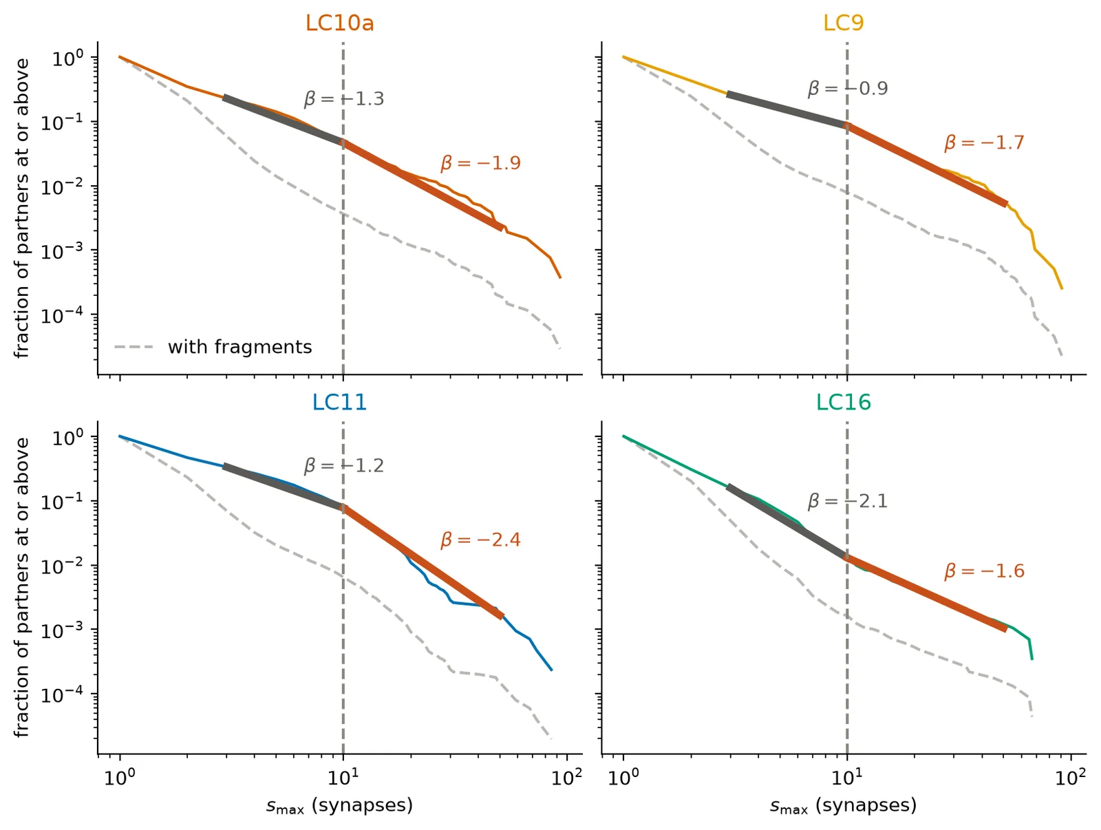
To read the bend directly, each panel draws the two chords of
BEND_MARKS on a type's \(s_{\mathrm{max}}\) curve for the proofread
partners, each labeled with its slope \(\beta\).
A curve that follows one straight line would give two chords with
the same slope.
The dashed curve counts the unproofread fragments as partners.
_fig, _axes = plt.subplots(2, 2, figsize=(8, 6), sharex=True, sharey=True)
_all_by_type = strengths_by_type(partners, "s_max")
_rows = []
for _ax, _t in zip(_axes.flat, TYPES_OF_INTEREST, strict=True):
    _all = ccdf(_all_by_type[_t])
    _ax.plot(
        _all["value"],
        _all["fraction"],
        color=CONTEXT_COLOR,
        linestyle="--",
        alpha=0.6,
        label="with fragments",
    )
    _curve = ccdf(s_max_by_type[_t])
    _ax.plot(_curve["value"], _curve["fraction"], color=TYPE_COLORS[_t])
    _fractions = [
        float((s_max_by_type[_t] >= _m).mean()) for _m in BEND_MARKS
    ]
    _slopes = local_slopes(s_max_by_type[_t], BEND_MARKS)[
        "slope"
    ].to_list()
    for _n, _color in enumerate((BULK_COLOR, TAIL_COLOR)):
        _xs, _ys = BEND_MARKS[_n : _n + 2], _fractions[_n : _n + 2]
        # Thicker than the curve so the chord stays visible on top
        # of it.
        _ax.plot(_xs, _ys, color=_color, linewidth=4)
        _ax.annotate(
            rf"$\beta = {_slopes[_n]:.1f}$",
            (np.sqrt(_xs[0] * _xs[1]), np.sqrt(_ys[0] * _ys[1])),
            xytext=(10, 8),
            textcoords="offset points",
            color=_color,
        )
    for _name, _frame in populations.items():
        _population_slopes = local_slopes(
            strengths_by_type(_frame, "s_max")[_t], BEND_MARKS
        )["slope"].to_list()
        _rows.append(
            {
                "type": _t,
                "population": _name,
                "bulk": _population_slopes[0],
                "tail": _population_slopes[1],
            }
        )
    _ax.axvline(STRONG_SYN, color=CONTEXT_COLOR, linestyle="--")
    _ax.set_xscale("log")
    _ax.set_yscale("log")
    _ax.set_title(_t, color=TYPE_COLORS[_t])
for _ax in _axes[1]:
    _ax.set_xlabel(r"$s_{\mathrm{max}}$ (synapses)")
for _ax in _axes[:, 0]:
    _ax.set_ylabel("fraction of partners at or above")
_axes[0, 0].legend(loc="lower left")
chord_slopes = pl.DataFrame(_rows).with_columns(
    flattening=pl.col("tail") - pl.col("bulk")
)
_fig
Two choices decide which partners the curve describes:
whether fragments count, and whether lateral partners (LC cells) do.
The dot plot shows the change of slope from the bulk chord to the
tail chord, the flattening, under every combination of the two.
A dot right of zero means the curve flattens above STRONG_SYN,
as a distinct strong group would make it;
a dot left of zero means it steepens.
add_population_legend keys the combinations to the marker shapes
and fills of POPULATION_MARKERS.
def add_population_legend(fig: Figure) -> None:
    """Add a key to fig for the marker of each population, drawn in
    gray because the type colors belong to the dots."""
    fig.legend(
        handles=[
            Line2D(
                [],
                [],
                color=CONTEXT_COLOR,
                marker=marker,
                markerfacecolor=CONTEXT_COLOR if filled else "white",
                linestyle="none",
                label=name,
            )
            for name, (marker, filled) in POPULATION_MARKERS.items()
        ],
        loc="outside right",
    )
_fig, _ax = plt.subplots(figsize=(7, 3.6))
_names = list(POPULATION_MARKERS)
for _n, _t in enumerate(TYPES_OF_INTEREST):
    for _m, _name in enumerate(_names):
        _marker, _filled = POPULATION_MARKERS[_name]
        _x = chord_slopes.filter(
            (pl.col("type") == _t) & (pl.col("population") == _name)
        )["flattening"].item()
        _ax.plot(
            _x,
            _n + 0.24 * (_m - 1.5),
            _marker,
            color=TYPE_COLORS[_t],
            markerfacecolor=TYPE_COLORS[_t] if _filled else "white",
        )
_ax.axvline(0, color=CONTEXT_COLOR, linestyle=":")
_ax.set_yticks(range(len(TYPES_OF_INTEREST)), TYPES_OF_INTEREST)
_ax.invert_yaxis()
_ax.set_xlabel("flattening: tail slope minus bulk slope")
add_population_legend(_fig)
_fig
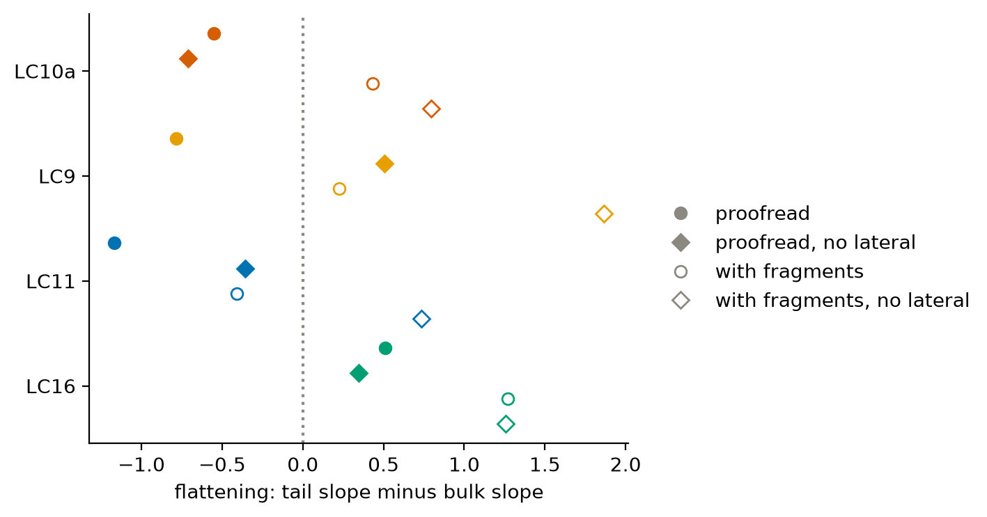
Flattening of the \(s_{\mathrm{max}}\) slope from the bulk chord to the tail chord (positive means less steep): proofread -1.2 to +0.5; proofread, no lateral -0.7 to +0.5; with fragments -0.4 to +1.3; with fragments, no lateral +0.7 to +1.9. The curve flattens in every type under 1 of the 4 combinations.
The local slopes of \(s_{\mathrm{max}}\) in the two intervals that
meet at STRONG_SYN, below it and above it:
_slopes = {
    _t: local_slopes(s_max_by_type[_t], SLOPE_MARKS)
    for _t in TYPES_OF_INTEREST
}
cutoff_slopes = pl.DataFrame(
    {
        "type": list(TYPES_OF_INTEREST),
        "below": [
            _s.filter(pl.col("upper") == STRONG_SYN)["slope"].item()
            for _s in _slopes.values()
        ],
        "above": [
            _s.filter(pl.col("lower") == STRONG_SYN)["slope"].item()
            for _s in _slopes.values()
        ],
    }
)
cutoff_slopes
| type | below | above |
|---|---|---|
| str | f64 | f64 |
| "LC10a" | -1.715168 | -1.696804 |
| "LC9" | -0.943601 | -1.616383 |
| "LC11" | -1.596808 | -2.569353 |
| "LC16" | -2.504634 | -1.653424 |
Where the data put the cutoff
The standard cutoff STRONG_SYN is a convention;
this section asks the data for a cutoff under each strength.
Both estimates use a grid of strengths spaced evenly on a log
scale, so that no mark is picked by hand.
Bend. Fit two straight lines joined at a knot to the log-log CCDF on the grid, trying each grid strength as the knot and keeping the one with the smallest squared error. The knot is where the slope changes. The Bayesian information criterion (BIC) compares this fit with a single line, and a positive gain favors a bend. Resampling the partners with replacement gives an interval for the knot.
Power law. A discrete power law \(p(s) \propto s^{-\alpha}\) is a straight line on the log-log curve, so the strength from which one fits the tail is another candidate for where the strong group begins. For each candidate start, fit \(\alpha\) by maximum likelihood to the partners at or above it, and measure the Kolmogorov-Smirnov distance, the largest gap between the data's CCDF and the fitted one. The start with the smallest distance wins.
log_grid returns the grid for a set of strengths:
whole numbers spaced evenly on a log scale,
from lower up to the largest strength that at least
min_partners partners reach.
For the proofread partners of LC10a under \(s_{\mathrm{max}}\):
def log_grid(
    strengths: ArrayLike,
    *,
    lower: int = 3,
    per_decade: int = 10,
    min_partners: int = 20,
) -> np.ndarray:
    """Whole-number strengths evenly spaced on a log scale from lower up
    to the largest strength that at least min_partners strengths reach.

    Raises ValueError when there are fewer than min_partners strengths.
    """
    ordered = np.sort(np.asarray(strengths))
    if len(ordered) < min_partners:
        msg = (
            f"log_grid needs at least {min_partners} strengths, "
            f"got {len(ordered)}"
        )
        raise ValueError(msg)
    top = ordered[-min_partners]
    steps = int(np.floor(per_decade * np.log10(top / lower)))
    return np.unique(
        np.rint(lower * 10 ** (np.arange(steps + 1) / per_decade))
    ).astype(int)
lc10a_s_max = strengths_by_type(proofread_partners, "s_max")["LC10a"]
lc10a_grid = log_grid(lc10a_s_max)
lc10a_grid
array([ 3, 4, 5, 6, 8, 9, 12, 15, 19, 24, 30])
Both fits below work on the log-log CCDF at the grid.
With \(x = \log_{10} m\) and \(y = \log_{10} F(m)\) for each grid
strength \(m\), with \(F\) from ccdf_at, the points for LC10a are:
lc10a_x = np.log10(lc10a_grid)
lc10a_y = np.log10(ccdf_at(lc10a_s_max, lc10a_grid))
pl.DataFrame({"x": lc10a_x, "y": lc10a_y})
| x | y |
|---|---|
| f64 | f64 |
| 0.477121 | -0.643189 |
| 0.60206 | -0.749443 |
| 0.69897 | -0.851242 |
| 0.778151 | -0.953748 |
| 0.90309 | -1.170196 |
| … | … |
| 1.079181 | -1.471226 |
| 1.176091 | -1.649764 |
| 1.278754 | -1.797366 |
| 1.380211 | -1.915466 |
| 1.477121 | -2.058888 |
line_squared_error is the squared error of the best single
straight line through the points, the baseline for a bend:
def line_squared_error(x: np.ndarray, y: np.ndarray) -> float:
    """Squared error of the least-squares straight line through the
    points (x, y)."""
    line = np.polyfit(x, y, 1)
    return float(((y - np.polyval(line, x)) ** 2).sum())
0.016422441244436953
fit_two_lines fits two straight lines that meet at a given knot
by least squares and returns their slopes and the squared error.
The knot is a position on the \(x\) axis, here the middle one:
class TwoLinesFit(NamedTuple):
    """Two straight lines that meet at a knot, fitted by least squares:
    the slope on each side of the knot and the squared error."""

    slope_below: float
    slope_above: float
    squared_error: float
def fit_two_lines(x: np.ndarray, y: np.ndarray, knot: float) -> TwoLinesFit:
    """The least-squares fit of two straight lines to the points (x, y)
    that meet at x = knot."""
    design = np.column_stack([np.ones_like(x), x, np.maximum(x - knot, 0)])
    coefficients = np.linalg.lstsq(design, y, rcond=None)[0]
    return TwoLinesFit(
        slope_below=float(coefficients[1]),
        slope_above=float(coefficients[1] + coefficients[2]),
        squared_error=float(((y - design @ coefficients) ** 2).sum()),
    )
TwoLinesFit(slope_below=-1.3696263047174735, slope_above=-1.6142292289510847, squared_error=0.012145061956299816)
bic scores a least-squares fit by its squared error and its
number of parameters; the smaller the better.
For the single line through the LC10a points:
def bic(squared_error: float, n: int, parameters: int) -> float:
    """Bayesian information criterion of a least-squares fit to n
    points with the given number of fitted parameters."""
    return float(n * np.log(squared_error / n) + parameters * np.log(n))
-66.7812290756555
fit_bend tries each grid strength as the knot of fit_two_lines,
keeps the knot with the smallest squared error,
and compares that fit with a single line by bic.
It leaves margin grid points on each side of a knot at least.
It returns a BendFit:
class BendFit(NamedTuple):
    """Two lines joined at a knot, fitted to a log-log CCDF.

    lowest_knot is the smallest grid strength tried as a knot, knot the
    grid strength where the two lines meet, and slope_below and
    slope_above their slopes.
    bic_gain is the BIC of one line minus the BIC of two lines, so it is
    positive when two lines fit better.
    """

    lowest_knot: int
    knot: float
    slope_below: float
    slope_above: float
    bic_gain: float
def fit_bend(
    strengths: ArrayLike, grid: np.ndarray, *, margin: int = 3
) -> BendFit:
    """The two-line fit to the log-log CCDF of strengths at the grid
    strengths, with the knot at the grid strength of smallest squared
    error.

    Raises ValueError when the grid has fewer than 2 * margin + 1
    strengths.
    """
    if len(grid) < 2 * margin + 1:
        msg = (
            f"the grid has {len(grid)} strengths; "
            f"a bend fit needs at least {2 * margin + 1}"
        )
        raise ValueError(msg)
    x = np.log10(grid)
    y = np.log10(ccdf_at(strengths, grid))
    knots = range(margin, len(grid) - margin)
    fits = [fit_two_lines(x, y, x[k]) for k in knots]
    best = min(range(len(fits)), key=lambda i: fits[i].squared_error)
    # Parameters: intercept and slope for one line; intercept, slope,
    # change of slope, and knot for two.
    one_line = bic(line_squared_error(x, y), len(grid), parameters=2)
    two_lines = bic(fits[best].squared_error, len(grid), parameters=4)
    return BendFit(
        lowest_knot=int(grid[margin]),
        knot=float(grid[knots[best]]),
        slope_below=fits[best].slope_below,
        slope_above=fits[best].slope_above,
        bic_gain=one_line - two_lines,
    )
BendFit(lowest_knot=6, knot=6.0, slope_below=-1.126697045505525, slope_above=-1.6124545516863455, bic_gain=6.696855144771476)
bootstrap_knots refits the bend on draws resamples of the
strengths, drawn with replacement, and returns the knot of each.
Their spread is the interval for the knot:
def bootstrap_knots(
    strengths: ArrayLike,
    grid: np.ndarray,
    *,
    draws: int = 200,
    seed: int = 0,
    margin: int = 3,
) -> np.ndarray:
    """The knot of fit_bend on each of draws resamples of strengths, on
    the same grid; the resamples come from a generator seeded with
    seed."""
    values = np.asarray(strengths)
    generator = np.random.default_rng(seed)
    resamples = (
        generator.choice(values, size=len(values)) for _ in range(draws)
    )
    return np.array(
        [fit_bend(sample, grid, margin=margin).knot for sample in resamples]
    )
array([6., 6., 6.])
For the power law, fit_exponent finds \(\alpha\) by maximum
likelihood for the strengths at or above a start.
Here the start is STRONG_SYN:
def fit_exponent(tail: ArrayLike, start: int) -> float:
    """The exponent of the discrete power law from start that the
    strengths in tail make most likely; tail holds the strengths at or
    above start."""
    values = np.asarray(tail)
    # Maximum likelihood on a fine grid of exponents;
    # 0.01 resolution is plenty for a distance comparison.
    alphas = np.linspace(1.01, 6.0, 500)
    negative_log_likelihood = len(values) * np.log(
        zeta(alphas, start)
    ) + alphas * float(np.log(values).sum())
    return float(alphas[np.argmin(negative_log_likelihood)])
lc10a_tail = lc10a_s_max.filter(lc10a_s_max >= STRONG_SYN)
lc10a_exponent = fit_exponent(lc10a_tail, STRONG_SYN)
lc10a_exponent
2.6500000000000004
ks_distance is the Kolmogorov-Smirnov distance between the CCDF
of those strengths and the CCDF of the power law with that
exponent:
def ks_distance(tail: ArrayLike, start: int, exponent: float) -> float:
    """The largest gap between the CCDF of the strengths in tail and
    the CCDF of the discrete power law from start with this exponent."""
    observed = ccdf(tail)
    modeled = zeta(exponent, observed["value"].to_numpy()) / zeta(
        exponent, start
    )
    return float(np.abs(observed["fraction"].to_numpy() - modeled).max())
0.04947342238219257
fit_power_law_from fits the power law to the strengths at or
above a start and returns a PowerLawFit:
class PowerLawFit(NamedTuple):
    """A discrete power law fitted to the strengths from start up.

    exponent is $\\alpha$ in $p(s) \\propto s^{-\\alpha}$, and distance
    is the Kolmogorov-Smirnov distance between the CCDF of the
    strengths and the fitted one.
    """

    start: int
    exponent: float
    distance: float
def fit_power_law_from(strengths: ArrayLike, start: int) -> PowerLawFit:
    """The discrete power law fitted to the strengths at or above
    start."""
    values = np.asarray(strengths)
    tail = values[values >= start]
    exponent = fit_exponent(tail, start)
    return PowerLawFit(
        start=int(start),
        exponent=exponent,
        distance=ks_distance(tail, start, exponent),
    )
PowerLawFit(start=10, exponent=2.6500000000000004, distance=0.04947342238219257)
fit_power_law tries every start from lowest_start up that
leaves at least min_tail strengths at or above it,
and keeps the fit with the smallest distance:
def fit_power_law(
    strengths: ArrayLike, *, lowest_start: int = 2, min_tail: int = 50
) -> PowerLawFit:
    """The fit of fit_power_law_from with the smallest distance over
    the starts from lowest_start up that leave at least min_tail
    strengths at or above them.

    Raises ValueError when no start leaves that many.
    """
    values = np.asarray(strengths)
    starts = [
        int(start)
        for start in np.unique(values[values >= lowest_start])
        if np.count_nonzero(values >= start) >= min_tail
    ]
    if not starts:
        msg = f"fewer than {min_tail} strengths are at or above {lowest_start}"
        raise ValueError(msg)
    return min(
        (fit_power_law_from(values, start) for start in starts),
        key=lambda fit: fit.distance,
    )
PowerLawFit(start=6, exponent=2.62, distance=0.018601244306713186)
cutoff_estimates gathers both estimates for one set of
strengths, with the 90% interval of the knot from bootstrap_knots:
class CutoffEstimates(NamedTuple):
    """Where a set of strengths puts the cutoff, by two methods.

    lowest_knot, knot, slope_below, slope_above, and bic_gain are the
    fields of the bend fit (BendFit), and knot_low and knot_high are
    the 5th and 95th percentiles of its knot over the resamples.
    power_law_start, exponent, and ks_distance are the start, exponent,
    and distance of the power-law fit (PowerLawFit).
    """

    lowest_knot: int
    knot: float
    knot_low: float
    knot_high: float
    slope_below: float
    slope_above: float
    bic_gain: float
    power_law_start: int
    exponent: float
    ks_distance: float
def cutoff_estimates(strengths: ArrayLike) -> CutoffEstimates:
    """The bend fit with a bootstrap interval for its knot, and the
    power-law fit, for one set of strengths."""
    grid = log_grid(strengths)
    bend = fit_bend(strengths, grid)
    knot_low, knot_high = np.quantile(
        bootstrap_knots(strengths, grid), [0.05, 0.95]
    )
    power = fit_power_law(strengths)
    return CutoffEstimates(
        lowest_knot=bend.lowest_knot,
        knot=bend.knot,
        knot_low=float(knot_low),
        knot_high=float(knot_high),
        slope_below=bend.slope_below,
        slope_above=bend.slope_above,
        bic_gain=bend.bic_gain,
        power_law_start=power.start,
        exponent=power.exponent,
        ks_distance=power.distance,
    )
CutoffEstimates(lowest_knot=6, knot=6.0, knot_low=6.0, knot_high=6.0, slope_below=-1.126697045505525, slope_above=-1.6124545516863455, bic_gain=6.696855144771476, power_law_start=6, exponent=2.62, ks_distance=0.018601244306713186)
cutoff_table runs cutoff_estimates for each strength, each
choice of partners, and each type.
Its column strength names the strength and partners the choice
of partners:
def cutoff_table(
    populations: dict[str, pl.DataFrame], columns: Sequence[str]
) -> pl.DataFrame:
    """The cutoff_estimates of each strength column among the partners
    of each type, for each choice of partners in populations.

    DataFrame[strength, type, partners, *fields of CutoffEstimates]:
    strength is the column and partners the key in populations.
    """
    return pl.DataFrame(
        [
            {
                "strength": column,
                "type": t,
                "partners": name,
                **cutoff_estimates(strengths)._asdict(),
            }
            for column in columns
            for name, partners in populations.items()
            for t, strengths in strengths_by_type(partners, column).items()
        ]
    )
| strength | type | partners | lowest_knot | knot | knot_low | knot_high | slope_below | slope_above | bic_gain | power_law_start | exponent | ks_distance |
|---|---|---|---|---|---|---|---|---|---|---|---|---|
| str | str | str | i64 | f64 | f64 | f64 | f64 | f64 | f64 | i64 | f64 | f64 |
| "s_max" | "LC10a" | "proofread" | 6 | 6.0 | 6.0 | 6.0 | -1.126697 | -1.612455 | 6.696855 | 6 | 2.62 | 0.018601 |
| "s_max" | "LC9" | "proofread" | 6 | 9.0 | 8.0 | 12.0 | -0.863093 | -1.587833 | 18.731328 | 10 | 2.64 | 0.03336 |
| "s_max" | "LC11" | "proofread" | 6 | 12.0 | 9.0 | 12.0 | -1.291802 | -3.461615 | 19.873066 | 12 | 3.78 | 0.042116 |
| "s_max" | "LC16" | "proofread" | 6 | 6.0 | 6.0 | 6.0 | -1.884691 | -2.575059 | 1.019092 | 4 | 3.02 | 0.042909 |
| "s_max" | "LC10a" | "proofread, no lateral" | 6 | 15.0 | 6.0 | 15.0 | -0.954324 | -1.250491 | 14.605195 | 2 | 2.03 | 0.034235 |
| … | … | … | … | … | … | … | … | … | … | … | … | … |
| "s_sum" | "LC16" | "with fragments" | 6 | 9.0 | 8.95 | 12.0 | -1.812927 | -0.960424 | 20.013003 | 2 | 2.42 | 0.017589 |
| "s_sum" | "LC10a" | "with fragments, no lateral" | 6 | 12.0 | 9.0 | 12.0 | -1.973085 | -0.576316 | 62.700574 | 2 | 2.81 | 0.020927 |
| "s_sum" | "LC9" | "with fragments, no lateral" | 6 | 15.0 | 12.0 | 15.0 | -2.072825 | -0.596384 | 54.460343 | 2 | 2.76 | 0.019592 |
| "s_sum" | "LC11" | "with fragments, no lateral" | 6 | 19.0 | 19.0 | 24.0 | -1.701577 | -0.744292 | 77.765179 | 2 | 2.55 | 0.00674 |
| "s_sum" | "LC16" | "with fragments, no lateral" | 6 | 15.0 | 12.0 | 19.0 | -1.848542 | -0.785514 | 71.977903 | 2 | 2.48 | 0.016543 |
_fig, _axes = plt.subplots(2, 2, figsize=(10, 7), sharey=True)
for _r, _column in enumerate(("s_max", "s_sum")):
    for _n, _t in enumerate(TYPES_OF_INTEREST):
        for _m, _name in enumerate(POPULATION_MARKERS):
            _marker, _filled = POPULATION_MARKERS[_name]
            _row = cutoffs.filter(
                (pl.col("strength") == _column)
                & (pl.col("type") == _t)
                & (pl.col("partners") == _name)
            ).row(0, named=True)
            _y = _n + 0.24 * (_m - 1.5)
            _face = TYPE_COLORS[_t] if _filled else "white"
            _axes[_r, 0].errorbar(
                _row["knot"],
                _y,
                xerr=[
                    [_row["knot"] - _row["knot_low"]],
                    [_row["knot_high"] - _row["knot"]],
                ],
                fmt=_marker,
                color=TYPE_COLORS[_t],
                markerfacecolor=_face,
            )
            _axes[_r, 1].plot(
                _row["power_law_start"],
                _y,
                _marker,
                color=TYPE_COLORS[_t],
                markerfacecolor=_face,
            )
for _r, _label in enumerate(
    (r"$s_{\mathrm{max}}$ (synapses)", r"$s_{\mathrm{sum}}$ (synapses)")
):
    for _c, _title in enumerate(
        ("knot of two lines (90% interval)", "start of the power-law fit")
    ):
        _ax = _axes[_r, _c]
        _ax.axvline(STRONG_SYN, color=CONTEXT_COLOR, linestyle="--")
        _ax.set_xscale("log")
        _ax.set_xticks(
            SLOPE_MARKS[1:], labels=[str(_m) for _m in SLOPE_MARKS[1:]]
        )
        _ax.minorticks_off()
        _ax.set_xlabel(_label)
        if _r == 0:
            _ax.set_title(_title)
    _axes[_r, 0].axvline(
        cutoffs["lowest_knot"].min(), color=CONTEXT_COLOR, linestyle=":"
    )
_axes[0, 0].set_yticks(range(len(TYPES_OF_INTEREST)), TYPES_OF_INTEREST)
_axes[0, 0].invert_yaxis()
add_population_legend(_fig)
_fig
The bend fit depends on its grid:
on the lowest strength the grid starts at (lower of log_grid)
and on the grid points kept on each side of a knot (margin of
fit_bend).
The knot of the proofread \(s_{\mathrm{max}}\) curves under each
pair of choices in GRID_STARTS and GRID_MARGINS:
grid_knots = pl.DataFrame(
    [
        {
            "type": _t,
            "grid starts at": _lower,
            "margin": _margin,
            "knot": fit_bend(
                s_max_by_type[_t],
                log_grid(s_max_by_type[_t], lower=_lower),
                margin=_margin,
            ).knot,
        }
        for _t in TYPES_OF_INTEREST
        for _lower in GRID_STARTS
        for _margin in GRID_MARGINS
    ]
)
grid_knots
| type | grid starts at | margin | knot |
|---|---|---|---|
| str | i64 | i64 | f64 |
| "LC10a" | 3 | 3 | 6.0 |
| "LC10a" | 3 | 2 | 5.0 |
| "LC10a" | 2 | 3 | 5.0 |
| "LC10a" | 2 | 2 | 5.0 |
| "LC9" | 3 | 3 | 9.0 |
| … | … | … | … |
| "LC11" | 2 | 2 | 10.0 |
| "LC16" | 3 | 3 | 6.0 |
| "LC16" | 3 | 2 | 5.0 |
| "LC16" | 2 | 3 | 5.0 |
| "LC16" | 2 | 2 | 4.0 |
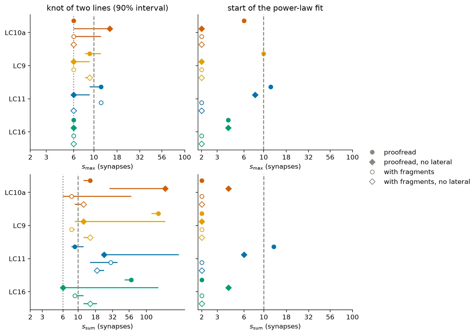
The dotted line marks 6 synapses, the lowest strength the fit tries as a knot. The best knot sits there in 11 of 16 for s_max, 1 of 16 for s_sum, so the bend is at or below it and the fit cannot place it.
Discussion
Summing admits more partners than the heaviest connection does. \(s_{\mathrm{sum}}\) calls strong 383 (LC10a), 341 (LC9), 686 (LC11), and 263 (LC16) proofread partners that \(s_{\mathrm{max}}\) does not, on top of the 122 (LC10a), 331 (LC9), 326 (LC11), and 37 (LC16) that both call strong. The partners strong by \(s_{\mathrm{sum}}\) only are connected to a median of 9% (LC9) to 35% (LC16) of the type's cells: the type reaches them together and no single cell does. Among the partners strong by \(s_{\mathrm{max}}\) that are not LC cells, the median partner is connected to 95% (LC16), 71% (LC11), 36% (LC10a), and 32% (LC9) of the type's cells. With the LC cells counted the medians are 27% (LC10a), 7% (LC9), 8% (LC11), and 93% (LC16).
The strong connections carry part of a strong partner's sum, and partners with more than one are common. For the strong proofread partners the median share of \(s_{\mathrm{sum}}\) that the strong connections carry is 36% (LC10a), 67% (LC9), 57% (LC11), and 41% (LC16), and 77 of 122 (LC10a), 162 of 331 (LC9), 104 of 326 (LC11), and 26 of 37 (LC16) have more than one strong connection. The CCDF of \(s_{\mathrm{sum,filtered}}\) flattens with strength: its local slope is -0.7 (LC10a), -0.9 (LC9), -1.6 (LC11), and -0.5 (LC16) in the first interval and -0.3 (LC10a), -0.3 (LC9), -0.3 (LC11), and -0.2 (LC16) in the last one with data, and the largest sums are 5,133 (LC10a), 1,598 (LC9), 2,505 (LC11), and 2,614 (LC16) synapses.
Expectation 1 for \(s_{\mathrm{max}}\): The slope changes near STRONG_SYN for LC9 and LC11 and not for LC10a and LC16. For proofread partners the best knots of two lines are LC10a at 6 (6 to 6), LC9 at 9 (8 to 12), LC11 at 12 (9 to 12), and LC16 at 6 (6 to 6) synapses (90% interval in parentheses), and the slope is steeper above the knot in every type. STRONG_SYN lies inside the interval for LC9 and LC11. For LC10a and LC16 the knot is the lowest strength the fit tries, and two lines beat one by a BIC of 1.0 (LC16) to 19.9 (LC11). Over all 16 combinations of type and partners, 11 knots sit at that lowest strength; flattening knots whose interval contains STRONG_SYN: 1. Among proofread partners a power law fits from 6 (LC10a), 10 (LC9), 12 (LC11), and 4 (LC16) synapses, with exponents of 2.6 (LC10a) to 3.8 (LC11); when fragments count it fits from 2 synapses.
Expectation 2 for \(s_{\mathrm{sum}}\): the knot lies higher than under \(s_{\mathrm{max}}\) for LC10a, LC9, and LC16, and the power law starts higher for LC11. For proofread partners the best knots are LC10a at 15 (12 to 15), LC9 at 150 (119 to 150), LC11 at 9 (8 to 12), and LC16 at 60 (48 to 60) synapses (90% interval in parentheses). Without lateral partners the intervals run from 6 to 300 synapses. Knots at the lowest strength: 1 of 16, against 11 of 16 under \(s_{\mathrm{max}}\). A power law fits from 2 (LC10a), 2 (LC9), 13 (LC11), and 2 (LC16) synapses, with exponents of 1.6 (LC10a) to 2.0 (LC11).
The local slope of \(s_{\mathrm{sum}}\) stays between -1.2 and -0.4 below 50 synapses, and changes by at most 0.2 between the intervals on the two sides of STRONG_SYN. No choice of strength puts the knot at STRONG_SYN for every type. Downstream work keeps the standard cutoff of lc_output_strength.
The chords flatten at the cutoff for only some choices of
partners.
The slope flattens above STRONG_SYN in every type under 1 of
the 4 choices of partners ("with fragments, no lateral").
Counting proofread neurons only, it steepens instead in
LC10a, LC9, and LC11
(Whether the slope changes at
the cutoff).
For LC9 and LC11 the local slope is steeper just above
STRONG_SYN than just below it,
so with LC cells counted there are fewer very strong partners than
one straight line would give, the opposite of a distinct strong
group.
The first expectation holds for the chords under 1 of the 4
choices of partners.
Limitations
The bend fit depends on its grid:
over the choices in GRID_STARTS and GRID_MARGINS,
the knot of the proofread \(s_{\mathrm{max}}\) curves moves
between LC10a 5 to 6, LC9 9 to 10, LC11 10 to 12, and LC16 4 to 6 synapses
(Where the data put the cutoff),
and the bootstrap treats partners as independent samples of the
curve, which they are not.
The slopes at the highest strengths rest on few partners.
\(s_{\mathrm{sum,filtered}}\) inherits the cutoff STRONG_SYN:
a lower one, such as the release paper's five synapses per
connection, would add connections and change every value.
Pooling retinotopic sub-groups (groups of cells whose dendrites
look at the same part of the visual field) can smooth a bend,
so the knots here describe the pooled curve.
A missing bend would not rule out two groups pooled together,
and a mixture of two populations produces a bend,
so a bend fits a strong set of real wiring without showing it.
Summing connections of one or two synapses also sums whatever false
positives they contain, which thresholding is meant to remove.
Open questions
- Are LC9's strong partners two kinds, cell-specific ones that a few cells connect to and type-wide ones that most cells connect to? Test: split them at, say, 10% and 50% of the type's cells and compare where the connected cells sit on the retinotopic grid. If the few-cell partners are connected to neighbors on the grid and the type-wide ones are not, the split is real.
- Does the number of cells in a type explain where the knot of \(s_{\mathrm{sum}}\) sits? A sum grows with the number of cells that can contribute. Test: divide \(s_{\mathrm{sum}}\) by the type's cell count and refit the knot. If the knots then agree across types, cell count explains the spread; if they still differ by a decade, it does not.
- Is the steep stretch below
STRONG_SYNmade of pieces of neurons that are already partners? Test: look up the current root of each fragment that gets two or more synapses from a type (CAVE keeps the edit history), merge the ones that join a proofread partner, and redraw the chords. If the bend stays away, the fragments were the cause. - Does a bend appear inside retinotopic sub-groups even though the
pooled curve has none?
Test: the CCDF of proofread partners per retinotopic bin or per
cluster of
lc_output_clusters. A sub-group whose bend sits away fromSTRONG_SYNsays the cutoff should be set per sub-group.
Terms
Each term is defined where it first appears; this list is for looking one up later.
- bend: a fairly sudden change of slope on the log-log CCDF, as when a second, heavier-tailed population takes over from the bulk.
- BIC (Bayesian information criterion):
how well a fit matches the data, penalized for each parameter it
uses.
bic_gainis the BIC of one line minus the BIC of two lines, so a positive gain favors a bend. - bootstrap interval: the middle 90% of a statistic (here the knot) over fits to the partners resampled with replacement.
- CCDF (complementary cumulative distribution function): the fraction of partners whose strength is at or above each value.
- chord: the straight line through two points of the CCDF on
log-log axes.
The bulk chord runs between the first two
BEND_MARKSand the tail chord between the last two. - connection: all the synapses from cell \(i\) to cell \(j\).
One synapse is enough here, as in the name of Codex's
connections_princeton_no_thresholdtable; the release paper calls two neurons connected only at five or more. - knot: the strength where the two lines of the bend fit meet.
- Kolmogorov-Smirnov distance: the largest gap between two cumulative distributions, here the CCDF of the data and the CCDF of a fitted power law.
- lateral partner: an LC cell that receives a connection from a cell of the type.
- local slope \(\beta(m_a, m_b)\): the slope of the log-log CCDF between two strengths.
- partner: a postsynaptic segment of a connection from some cell of a type, either a proofread neuron or an unproofread fragment. LC cells count.
- power law: a distribution whose CCDF is a straight line on log-log axes. For whole numbers \(p(s) \propto s^{-\alpha}\), and \(\alpha\) is the exponent.
- proofread neuron: a segment that people have proofread and
joined into a neuron (
proofread_ids). - retinotopic: arranged like the retina, so that neighboring cells look at neighboring points of the visual field.
- \(s_{\mathrm{max}}\) (strength): the weight of the heaviest single connection from a cell of the type onto a partner.
- \(s_{\mathrm{sum}}\) (strength): the number of synapses from all cells of the type onto a partner.
- \(s_{\mathrm{sum,filtered}}\) (strength): the number of synapses in the strong connections from cells of the type onto a partner; 0 for a partner with none.
- strong by a strength: a partner whose value of that strength
is at or above
STRONG_SYN. - strong connection: a connection of at least
STRONG_SYNsynapses. - unproofread fragment: an automated segment that is not a proofread neuron.
- weight \(w(i \to j)\): the number of synapses in the connection from \(i\) to \(j\).